April 17th, 2017 • Comments Off on Distributed systems: which cluster do I obey?
The topic of cluster formation in itself is not new. There are plenty of methods around to form cluster on the fly [1]. They mostly follow methods which make use of gossip protocols. Implementation can wildly be found, even in products like Akka.
Once a cluster is formed the question becomes wehter control (see this post for some background) is centralized or decentralized. Or something in between with a (hierarchical) set of leaders managing – in a distributed fashion – a cluster of entities that are actuating. Both, centralized and decentralized approaches, have their advantages and disadvantages. Centralized approaches are sometimes more efficient as they might have more knowledge to base their decisions upon. Note that even in centralized management approaches a gossip protocols might be in use. There are also plenty of algorithms around to support consensus and leader election [2], [3].
Especially in Fog and Fdge computing use cases, entities which move (e.g. a car, plane, flying/sailing drone) have to decide to which cluster they want to belong and obey the actions initiated by those. Graph representations are great for this – and yet again because of a rich set of algorithms in the graph theory space, the solution might be quite simple to implement. Note that in Fog/Edge use cases there most likely will always be very (geographic) static entities like Cloudlets in the mix – which could be elected as leaders.
For example, the following diagram shows two clusters: The red nodes’ size indicates who is the current leader. The blue dot – marks an entity that is connected to both clusters. The width of the edge connecting it to the cluster indicates to which cluster it ‘belongs’ (aka it’s affinity).
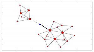
(Click to enlarge)
Now as the blue entity moves (geographically) the connections/edges to the clusters change. Now based on algorithms like this, the entity can make a decision to hand-off control to another cluster and obey the directions given from it.
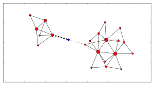
(Click to enlarge)
Categories: Personal • Tags: Distributed Systems, Graphs • Permalink for this article
January 7th, 2017 • Comments Off on Example 2: Intelligent Orchestration & Scheduling with OpenLava
This is the second post in a series (the first post can be found here) about how to insert smarts into a resource manager. So let’s look how a job scheduler or distributed resource management system (DRMS) — in a HPC use case — with OpenLava can be used. For the rationale behind all this check the background section of the last post.
The basic principle about this particular example is simple: each host in a cluster will report a “rank”; the rank will be used to make a decision on where to place a job. The rank could be defined as: a rank is high when the sub-systems of the hosts are heavily used; and the rank is low when none or some sub-system are utilized. How the individual sub-systems usage influences the rank value, is something that can be machine learned.
Let’s assume the OpenLava managed cluster is up and running and a couple of hosts are available. The concept of elims can be used to get the job done. The first step is, to teach the system what the rank is. This is done in the lsf.shared configuration file. The rank is defined to be a numeric value which will be updated every 10 seconds (while not increasing):
Begin Resource
RESOURCENAME  TYPE    INTERVAL INCREASING  DESCRIPTION
   ...
   rank       Numeric 10       N           (A rank for this host.)
End Resource
Next OpenLava needs to know for which hosts this rank should be determined. This is done through a concept of ‘resource mapping’ in the lsf.cluster.* configuration file. For now the rank should be used for all hosts by default:
Begin ResourceMap
RESOURCENAME LOCATION
rank ([default])
End ResourceMap
Next an external load information manager (LIM) script which will report the rank to OpenLava needs to be written. OpenLava expects that the script writes to stdout with the following format: <number of resources to report on> <first resource name> <first resource value> <second resource name> <second resource value> … . So in this case it should spit out ‘1 rank 42.0‘ every 10 seconds. The following python script will do just this – place this script in the file elim in $LSF_SERVERDIR:
#!/usr/bin/python2.7 -u

import time

INTERVAL = 10


def _calc_rank():
    # TODO calc value here...
    return {'rank': value}

while True:
    RES = _calc_rank()
    TMP = [k + ' ' + str(v) for k, v in RES.items()]
    print(\"%s %s\" % (len(RES), ' '.join(TMP)))
    time.sleep(INTERVAL)
Now a special job queue in the lsb.queues configuration file can be used which makes use of the rank. See the RES_REQ parameter in which it is defined that the candidate hosts for a job request are ordered by the rank:
Begin Queue
QUEUE_NAME = special
DESCRIPTION = Special queue using the rank coming from the elim.
RES_REQ = order[rank]
End Queue
Submitting a job to this queue is as easy as: bsub -q special sleep 1000. Or the rank can be passed along as a resource requirements on job submission (for any other queue): bsub -R “order[-rank]” -q special sleep 1000. By adding the ‘-‘ it is said that the submitter request the candidate hosts to be sorted for hosts with a high rank first.
Let’s assume a couple of hosts are up & running and they have different ranks (see the last column):
openlava@242e2f1f935a:/tmp$ lsload -l
HOST_NAME               status  r15s   r1m  r15m   ut    pg    io  ls    it   tmp   swp   mem   rank
45cf955541cf                ok   0.2   0.2   0.3   2%   0.0     0   0 2e+08  159G   16G   11G    9.0
b7245f8e6d0d                ok   0.2   0.2   0.3   2%   0.0     0   0 2e+08  159G   16G   11G    8.0
242e2f1f935a                ok   0.2   0.2   0.3   3%   0.0     0   0 2e+08  159G   16G   11G   98.0
When checking the earlier submitted job, the execution host (EXEC_HOST) is indeed the hosts with the lowest rank as expected:
openlava@242e2f1f935a:/tmp$ bjobs
JOBID   USER    STAT  QUEUE      FROM_HOST   EXEC_HOST   JOB_NAME   SUBMIT_TIME
101     openlav RUN   special    242e2f1f935 b7245f8e6d0 sleep 1000 Jan  7 10:06
The rank can also be seen in web interface like the one available for the OpenLava Mesos framework. What was described in this post is obviously just an example – other methods to integrate your smarts into the OpenLava resource manager can be realized as well.
Categories: Personal • Tags: LSF, Orchestration, Scheduling, SDI • Permalink for this article
September 18th, 2016 • Comments Off on Example 1: Intelligent Orchestration & Scheduling with Kubernetes
In the last blog I suggested that analytical capabilities need to move to the core of resource managers. This is very much needed for autonomous controlled large scale systems which figure out the biggest chunk of decisions to be made themselves. While the benefits from this might be obvious, the how to inject the insights/intelligence back into the resource manager might not be. Hence this blog post series documenting a bit how to let systems (they are just examples – trying to cover most domains :-)) like Kubernetes, OpenStack, Mesos, YARN and OpenLava make smarter decisions.
Background
The blog posts are going to cover some generic concepts as well as point to specific documentation bits of the individual resource managers. Some of this is already covered in past blog posts but to recap let’s look at the 5(+1) Ws for resource managers decision making (click to skip to the technical details):
- What decision needs to be made? – Decisions – and the actuations they lead too – can roughly be categorized into: doing initial placement of workloads on resources, the re-balancing of workload and resource landscapes (through either pausing/killing, migrating or tuning resource and workloads) and capacity planning activities (see ref).
- Who is involved? – The two driving forces for data center resource management are the customer and the provider. The customer looking for good performance and user experience while the provider looking for maximizing his ROI & lowering TCO of his resources. The customer is mostly looking for service orchestration (e.g. doesn’t care where and how the workload runs, as long as it performs and certain policies and rules – like for auto-scaling are adhered; or see sth like google’s instance size recommendation feature) while the provider looks at infrastructure orchestration of larger scale geo-distributed infrastructures (and the resources within) with multiple workloads from different customers (tenants are not equal btw – some are low playing non important workloads/customers some high paying important workloads/customers with priorities and SLAs).
- When does the decision/actuation apply? – Decisions can either be made immediately (e.g. an initial placement) or be more forward/backward looking (e.g. handle a maintenance/forklift upgrade request for certain resources).
- Where does the decision need to be made?- This is probably one of the most challenging questions. First of all this covers the full stack from physical resources (e.g. compute hosts, air-conditioning, …), software defined resources (e.g. virtual machines (VM), containers, tasks, …) all the way to the services the customers are running, as well as across domains of compute (e.g CPUs, VMs, containers, …), network (e.g. NICs, SDN, …) and storage (e.g. Disks, block/object storage, …). Decisions are done on individual resource, aggregated, group, data center or a global level. For example the NIC, the Virtual machine/container/tasks hosting the workload, or even the power supply can be actuated upon (feedback control is great for this). The next level actuations can be carried out on the aggregate level – in which a set of resources make up a compute hosts, ToR-switch, SAN (e.g. by tuning the TCP/IP stack in the kernel). Next up is the group level for which e.g. polices across a set of aggregates can be defined (e.g. over-subscription policy for all Xeon E5 CPUs, a certain rack determined to run small unimportant jobs vs. a rack needing to run high performance workloads). Next is the data center level for which we possibly want to enforce certain efficiency goals driven by business objective (e.g. lowering the PuE). Finally the global level captures possible multiple distributed data centers for which decisions need to be made which enable e.g. high availability and fault tolerance.
- Why does the decision need to be made? Most decision are made for efficiency reasons derived from business objectives of the provider and customer. This means ultimately the right balance between the customer deploying the workload and asking for performance and SLA compliance (customers tend to walk away if the provider doesn’t provide a good experience) and the provider improving TCO (not being able to have a positive cashflow normally lead to a provider running out of business).
- How is the decision/actuation made? This is the focus for this article series. In case it is determined a decision needs to be made, it needs to be clear on how to carry out the actual actuation(s) for all the kinds of decision that can be made described above.
Decision most of the time cannot be made generic – e.g. decisions made in HPC/HTC systems do not necessarily apply to a telco environments in which the workloads and resource are different. Hence the context of workloads and resource in place play a huge role. Ultimately Analytics which embraces the context (in all sorts and forms: deep/machine learning, statistical modelling, artificial intelligence, …) of the environment can drive the intelligence in the decision making through insights. This can obviously in multiple places/flows (see the foreground and background flow concepts here) and ultimately enables autonomous control.
Enhancing Kubernetes
For the Kubernetes examples let’s focus on a crucial decision point – doing the initial placement of a workloads (aka a POD in Kubernetes language) in a cluster. Although much of today’s research focuses on initial placement I’d urge everybody not to forget about all the other decisions that can be made more intelligent.
Like most Orchestrators and Schedulers Kubernetes follows a simple approach of filtering and ranking. After shortlisting possible candidates, the first step involves filtering those resource which do not meet the workloads demands. The second step involves prioritization (or ranking) of the resources best suited.
This general part is described nicely in the Kubernetes documentation here: https://github.com/kubernetes/kubernetes/blob/master/docs/devel/scheduler.md
This filtering part is mostly done based on capacities, while the second can involve information like the utilization. If you want to see this code have a look at the generic scheduling implementation: here. The available algorithms for filtering (aka predicates) and prioritization can be found here. The default methods that Kubernetes filters upon can be seen here: here – the default prioritization algorithms here: here. Note that weights can be applied to the algorithms based on your own needs as a provider. This is a nice way to tune and define how the resource under the control of the provider can be used.
While the process and the defaults already do a great job – let’s assume you’ve found a way on when and how to use an accelerator. Thankfully like most scheduling systems the scheduler in Kubernetes is extendable. Documentation for this can be found here. 3 ways are possible:
- recompile and alter the scheduler code,
- implement your own scheduler completely and run it in parallel,
- or implement an extension which the default scheduler calls when needed.
The first option is probably hard to manage in the long term, the second option requires you to deal with the messiness or concurrency while the third option is interesting (although adds latency to the process of scheduling due to an extra HTTP(s) call made). The default scheduler can basically call an external process to either ‘filter’ or ‘prioritize’. In the first case a list of possible candidate hosts is returned, in the the second case a prioritized list if returned. Now unfortunately the documentation get’s a bit vague, but luckily some code is available from the integration tests. For example here you can see some external filtering code, and here the matching prioritization code. Now that just needs to be served up over HTTP and you are ready to go, next to adding some configurations documented here.
So now an external scheduler extension can make a decisions if an accelerator should be assigned to a workload or not. The intelligent decision implemented in this extender could e.g. decide if an SR-IOV port is needed based on a bandwidth requirement, or if it is even a good idea to assign a Accelerator to a workload par the previous example.
Corrections, feedback and additional info are more then welcome. I’ve some scheduler extender code running here – but that is not shareable yet. I will update the post once I’ve completed this. In the next posts OpenStack (e.g. service like Nova, Watcher, Heat and Neutron), Mesos (how e.g. allocator modules can be used to inject smarts) and OpenLava (for which e.g. elims can be used to make better scheduling decisions) and obviously others will be introduced 🙂
Categories: Personal • Tags: Orchestration, Scheduling, SDI • Permalink for this article
July 25th, 2016 • Comments Off on Insight driven resource management & scheduling
Future data center resource and workload managers – and their [distributed]schedulers – will require a new key integrate capability: analytics. Reason for this is the the pure scale and the complexity of the disaggregation of resources and workloads which requires getting deeper insights to make better actuation decisions.
For data center management two major factors play a role: the workload (processes, tasks, containers, VMs, …) and the resources (CPUs, MEM, disks, power supplies, fans, …) under control. These form the service and resource landscape and are specific to the context of the individual data center. Different providers use different (heterogeneous) hardware (revisions) resource and have different customer groups running different workloads. The landscape overall describes how the entities in the data center are spatially connected. Telemetry systems allow for observing how they behave over time.
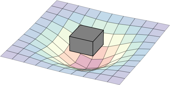
The following diagram can be seen as a metaphor on how the two interact: the workload create a impact on the landscape. The box represent a simple workload having an impact on the resource landscape. The landscape would be composed of all kind of different entities in the data center: from the air conditioning facility all the way to the CPU. Obviously the model taken here is very simple and in real-life a service would span multiple service components (such as load-balancers, DBs, frontends, backends, …). Different kinds of workloads impact the resource landscape in different ways.

(Click to enlarge)
Current data center management systems are too focused on understanding resources behavior only and while external analytics capabilities exists, it becomes crucial that these capabilities need to move to the core of it and allow for observing and deriving insights for both the workload and resource behavior:
- workload behavior: Methodologies such as described in this paper, become key to understand the (heterogeneous) workload behavior and it’s service life-cycle over space and time. This basically means learning the shape of the workload – think of it as the form and size of the tile in the game Tetris.
- resource behavior: It needs to be understood how a) heterogeneous workloads impact the resources (especially in the case of over-subscription) and b) how features of the resource can impact the workload performance. Think of the resources available as the playing field of the game Tetris. Concept as described in this paper help understand how features like SR-IOV impact workload performance, or how to better dimension the service component’s deployment.
Deriving insights on how workloads behave during the life-cycle, and how resources react to that impact, as well as how they can enhance the service delivery is ultimately key to finding the best match between service components over space and time. Better matching (aka actually playing Tetris – and smartly placing the title on the playing field) allows for optimized TCO given a certain business objective. Hence it is key that the analytical capabilities for getting insights on workload and resource behavior move to the very core of the workload and resource management systems in future to make better insightful decisions. This btw is key on all levels of the system hierarchy: on single resource, hosts, resource group and cluster level.
Note: parts of this were discussed during the 9th workshop on cloud control.
Categories: Personal • Tags: Analytics, Cloud, data center, Machine Learning, Orchestration, Scheduling, SDI • Permalink for this article
March 24th, 2016 • Comments Off on A data center resource and service landscape
Telemetry and Monitoring systems give a great visibility into what is going on with the resources and services in a data center. Applying machine learning and statistical analysis to this massive data source alone often leads to results where it becomes clear correlation ain’t causation.
This brings the need for understanding of “what is connected to what” in a data center. By adding this topology as a data source, it is much easier to understand the relationships between two entities (e.g. a compute node and it’s Container/VM or a block storage and the NAS hosting it).
One of the ultimate goals we have here in Intel Labs is to put the data center on autopilot and hence we try to answer the Q:
how to efficiently define and maintain a physical and logical resource and service landscape enriched by operational/telemetry data, to support orchestration for optimized service delivery
We have therefore come up with a landscape graph model. The graph model captures all the entities in a data center/SDI and makes their relations explicit. The following diagram shows the full-stack (from physical to virtual to service entities) landscape of a typical data center.
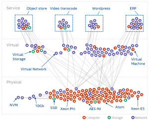
(Click to enlarge)
The graph model is automatically derived from systems such as OpenStack (or similar) and allow us to run all kinds of analytics – especially when we combine the graph model and annotate it with with data from telemetry systems.
As one example use case for using the landscape and annotate it with telemetry data, this paper shows a way to colour the landscape for anomaly detection.
Categories: Work • Tags: Cloud, data center, Orchestration, Scheduling, SDI • Permalink for this article
Page 3 of 36«12345...102030...»Last »


