June 14th, 2020 • Comments Off on AI planning algorithms in Rust
Artificial Intelligence (AI) is a hot topic, although it seams that the focus is on Neural Networks & Deep Learning on the software/algorithmic side, while GPUs/TPUs are the #1 topic for hardware. While this is fine, it feels sometimes like other parts of what had been part of the overall AI domain in the past fall short (See the book Artificial Intelligence: A Modern Approach). Just by looking at the table of contents you can see many more AI topics which are critical but do not get a lot of attention atm. For example planning & reasoning over the insight you have gained – by e.g. using neural networks – is essential to build “semi-cognitive” autonomous systems. Btw I believe planning (the what/how) is as important as figure out the scheduling (when/where) – for example AlphaGo Zero also uses a planning component (using Monte Carlo tree search) for figuring out the next move – next to a neural network.
To have an excuse to learn Rust and to get more into planning & reasoning algorithms I started developing this library (Warning: this is still a work in progress). The experience with Rust and its ecosystem have been great so far. The Ownership concept takes some time to get used to, and probably only makes total sense after a while. A lot of the other concepts can also be found in other languages, so that makes starting easy.
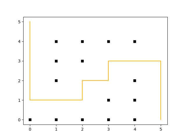
The following example shows the D* Lite algorithm in action. Assume you have a maze like the one shown in the following figure and the goal is to move a robot from the coordinates (5, 0) to (0, 5). To make things more complicated, we assume a path along the corners of the maze is more “expensive” – so at the start the path a robot could take looks like this:
(Click to enlarge)
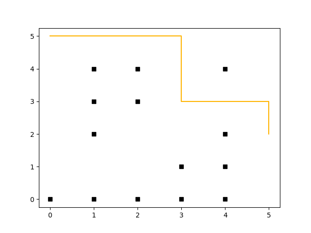
In contrast to A*, D* Lite uses a backward search and enables re-planning – that means that after e.g. the robot has moved two steps (to coordinate (5, 2)), and an obstacle gets removed (coordinate (3, 4) no longer represents a wall) it can re-plan without the need to recalculate all values (saving compute time). This can be seen in the following diagram (both diagrams have been plotted through rustplotlib by using Matplotlib in the background, btw. – this shows how easy it is to integrate Python with Rust.):
(Click to enlarge)
Why Rust? Over the years I learned some programing languages, some probably gone extinct by now. This includes candidates such as Oberon, Turbo Pascal (anyone remember Turbo Vision?), Elan, and Basic. I used to code in Java & C/C++ for a while – today it is more Python and a little bit of Go. It has been nagging me for a while, that I wanted to learn a language that was somehow “revolutionary” and offered sth new. For example Java is a great language & has a powerful SDK; Python is easy to use; etc. But Rust finally offered something new – the concepts around its memory management (w/o the need for garbage collection) & the way that it enforces you to write clean code are compelling (Maybe we can finally battle cargo cult programming). I have looked into Erlang too btw, but the syntax is just a bit too quirky – however the OTP is a very strong concept and sometimes it feels like that Cloud Native Applications + Kubernetes want to be the future OTP 🙂 Microsoft btw also describes some of their motivations to use Rust here.
So Rust is perfect? Probably not (yet) – many tools/libraries in the ecosystem are still young (e.g. grcov works only with nightly toolchain), and do not offer the same range of capabilities as e.g. in the Python world (still looking for good machine learning library etc. for example). Getting to know Rust is a bit painful in the beginning – and one word of advice: do not always follow the tips from the compiler, which it spews out on errors – sit back, think about what the errors actually means and fix it accordingly.
Any Book suggestions? So for learning Rust I mostly went with the “official” Rust book and got an older hardcopy of the book (the last programming books I bought before this was on Erlang years ago btw.). I heard the O’Reilly book on Rust is great too btw.
Categories: Personal • Tags: Algorithm, Artificial Intelligence, Autonomic System, Rust • Permalink for this article
January 4th, 2020 • Comments Off on AI reasoning & planning
With the rise of faster compute hardware and acceleration technologies that drove Deep Learning, it is arguable that the AI winters are over. However Artificial Intelligence (AI) is not all about Neural Networks and Deep Learning in my opinion. Even by just looking at the table of contents of the book “AI – A modern approach” by Russel & Norvig it can easily be seen, that the learning part is only one piece of the puzzle. The topic of reasoning and planning is equally – if not even more – important.
Arguably if you have learned a lot of cool stuff you still need to be able to reason over that gained knowledge to actually benefit from the learned insights. This is especially true, when you want to build autonomic systems. Luckily a lot of progress has been made on the topic of automated planning & reasoning, although they do not necessarily get the same attention as all the neural networks and Deep Learning in general.
To build an autonomous systems it is key to use these kind of techniques which allow for the system to adapt to changes in the context (temporal or spatial changes). I did work a lot on scheduling algorithms in the past to achieve autonomous orchestration, but now believe that planning is an equally important piece. While scheduling tells you where/when to do stuff, planning tells you what/how to do it. The optimal combination of scheduling and planning is hence key for future control planes.
To make this more concrete I spend some time implementing planning algorithms to test concepts. Picture the following, let’s say you have two robot arms. And you just give the control system the goal to move a package from A to B you want the system to itself figure out how to move the arms, to pick the package up & move it from A to B. The following diagram shows this:
 (Click to enlarge & animate)
The goal of moving the package from A to B is converted into a plan by looking at the state of the packages which is given by it’s coordinates. By picking up the package and moving it around the state of the package hence changes. The movement of the robot arms is constraint, while the smallest part of the robot arm can move by 1 degree during each time step the bigger parts of the arm can move by 2 & 5 degrees respectively.
Based on this, a state graph can be generated. Where the nodes of the graph define the state of the package (it’s position) and the edges actions that can be performed to alter those states (e.g. move a part of an robot arm, pick & drop package etc.). Obviously not all actions would lead to an optimal solution so the weights on the edges also define how useful this action can be. On top of that, an heuristic can be used that allows the planning algorithm to find it’s goal faster. To figure out the steps needed to move the package from A to B, we need to search this state graph and the “lowest cost” path between start state (package is at location A) and end state (package is at location B) defines the plan (or the steps on what/how to achieve the goal). For the example above, I used D* Lite.
Now that a plan (or series of step) is known we can use traditional scheduling techniques to figure out in which order to perform these. Also note the handover of the package between the robots to move it from A to B this shows – especially in distributed systems – that coordination is key. More on that will follow in a next blog-post.
Categories: Personal • Tags: Algorithm, Artificial Intelligence, Autonomic System, Distributed Systems, Machine Learning, Planning • Permalink for this article
January 20th, 2019 • Comments Off on Dancing links, algorithm X and the n-queens puzzle
Donald Knuth’s 24th annual Christmas lecture inspired me to implement algorithm X using dancing links myself. To demonstrate how this algorithms works, I choose the n-queens puzzle. This problem has some interesting aspects to it which show all kinds of facets of the algorithm.
Solving the n-queens puzzle using algorithm X can be achieved as follows. Each queen being placed on a chess board will lead to 4 constraints that need to be cared for:
- There can only be one queen in the given row.
- There can only be one queen in the given column.
- There can only be one queen in the diagonal going from top left to bottom right.
- There can only be one queen in the diagonal going from bottom left to top right.
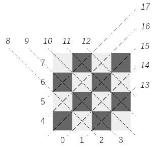
Let’s look at a chess board and determine some identifiers for each constraint that any placement can have (See the youtube video of the lecture at this timestep). Donald Knuth doesn’t go into too many details on how to solve this but let’s look at an 4×4 chessboard example:
 (Click to enlarge)
Assigning an identifier can be done straight forward: column based constraints are numbered 0-3; row based constraints get the ids from 4-7; diagonals 8-12; reverse diagonals 13-17 for a chessboard of size 4. Note that you can ignore the diagonal of size 1, as they are automatically covered by the row or column the queen would be placed in.
Calculating the identifiers for the constraints is simple. Given an queen positioned at coordinates (x, y) on a chessboard of size N these are the formulations you can use:
- the row constraint equals x
- the column constraint equals y + N
- for the diagonal constraint equals x + y + (2N-1)
- for the reverse diagonal constraint equals (N – 1 – x + y) + (4N-4)
Note that each constraint identifier calculation we use an offset, so we can all represent them in one context: 0 for the row constraints, N for the column constraints, 2N-1 for the diagonal and 4N-4 for the reverse diagonal constraints. For the diagonal constraints you need to ensure they are within their ranges: 2*N-1 < constraint < 3*N and 3*N+1 < constraint < 4*N + 1. If the calculated identifier of the constraints is not within the ranges, you can just drop the constraint – this is the case for queens being placed at corner positions. Placing a queen at coordinates (0,0) will result in 3 constraints: [0, 4, 15]. Placing a queen at coordinates (1,2) will results in 4 constraints: [1, 6, 10, 16].
Now that for each queen that can be placed we can calculate the uniquely identifiable constraints identifier, we can translate this problem into an exact cover problem. We are looking for a set of placed queens, for which all constraints can be satisfied. Let’s look at a matrix representation (for a chessboard of size 4, in which the rows are individual possible placements options of a queen, while the columns represent the constraints. The 1s indicate that it is a constraint that needs to be satisfied for the given placement.
| Queen coordinates | Primary constraints | Secondary constraints |
| x-coord | y-coord | diagonals | r-diagonals |
| 0 | 1 | 2 | 3 | 4 | 5 | 6 | 7 | 8 | 9 | 10 | 11 | 12 | 13 | 14 | 15 | 16 | 17 |
| 0,0 | 1 | | | | 1 | | | | | | | | | | | 1 | | |
| 0,1 | 1 | | | | | 1 | | | 1 | | | | | | | | 1 | |
| 0,2 | 1 | | | | | | 1 | | | 1 | | | | | | | | 1 |
| 0,3 | 1 | | | | | | | 1 | | | 1 | | | | | | | |
1,0
| | 1 | | | 1 | | | | 1 | | | | | | 1 | | | |
| 1,1 | | 1 | | | | 1 | | | | 1 | | | | | | 1 | | |
| 1,2 | | 1 | | | | | 1 | | | | 1 | | | | | | 1 | |
| 1,3 | | 1 | | | | | | 1 | | | | 1 | | | | | | 1 |
| 2,0 | | | 1 | | 1 | | | | | 1 | | | | 1 | | | | |
| 2,1 | | | 1 | | | 1 | | | | | 1 | | | | 1 | | | |
| 2,2 | | | 1 | | | | 1 |
| | | | 1 | | | | 1 | | |
| 2,3 | | | 1 | |
| | | 1 | | | | | 1 | | | | 1 | |
| 3,0 | | | | 1 | 1 |
| | | | | 1 | | | | | | | 1 |
| 3,1 | | | | 1 | | 1 |
| | | | | 1 | | 1 | | | | |
| 3,2 | | | | 1 | | | 1 | | | | | | 1 | | 1 | | | |
| 3,3 | | | | 1 | | | | 1 | | | | | | | | 1 | | |
Note that the table columns have been grouped into two categories: primary and secondary constraints. This is also a lesser known aspect of the algorithms at hand – primary columns and their constraints must be covered exactly once, while the secondary columns must only be covered at most once. Looking at the n-queens puzzle, this make sense – to fill the chessboard to the maximum possible number of queens, each row and column should have a queen, while there might be diagonals which are not blocked by a queen.
Implementing algorithm x using dancing links is reasonable simple – just follow the instructions in Knuth’s paper here. Let’s start with some Go code for the data structures:
type x struct {
	left  *x
	right *x
	up    *x
	down  *x
	col   *column
	data  string
}

type column struct {
	x
	size int
	name string
}

type Matrix struct {
	head      *x
	headers   []column
	solutions []*x
}
Note the little change I made to store a data string in the object x structure. This will be useful when printing the solutions later on. The following function in the can be used to initialize a new matrix:
func NewMatrix(n_primary, n_secondary int) *Matrix {
	n_cols := n_primary + n_secondary

	matrix := &Matrix{}
	matrix.headers = make([]column, n_cols)
	matrix.solutions = make([]*x, 0, 0)
	matrix.head = &x{}
	matrix.head.left = &matrix.headers[n_primary-1].x
	matrix.head.left.right = matrix.head

	prev := matrix.head
	for i := 0; i < n_cols; i++ {
		column := &matrix.headers[i]
		column.col = column
		column.up = &column.x
		column.down = &column.x
		if i < n_primary {
			// these are must have constraints.
			column.left = prev
			prev.right = &column.x
			prev = &column.x
		} else {
			// as these constraints do not need to be covered - do not weave them in.
			column.left = &column.x
			column.right = &column.x
		}
	}
	return matrix
}
Now that we can instantiate the matrix data structure according to Knuth's description the actual search algorithm can be run. The search function can roughly be split into 3 parts: a) if we found a solution - print it, b) finding the next column to cover and c) backtrack search through the remaining columns:
func (matrix *Matrix) Search(k int) bool {
	j := matrix.head.right
	if j == matrix.head {
		// print the solution.
		fmt.Println("Solution:")
		for u := 0; u < len(matrix.solutions); u += 1 {
			fmt.Println(u, matrix.solutions[u].data)
		}
		return true
	}

	// find column with least items.
	column := j.col
	for j = j.right; j != matrix.head; j = j.right {
		if j.col.size < column.size {
			column = j.col
		}
	}

	// the actual backtrack search.
	cover(column)
	matrix.solutions = append(matrix.solutions, nil)
	for r := column.down; r != &column.x; r = r.down {
		matrix.solutions[k] = r
		for j = r.right; j != r; j = j.right {
			cover(j.col)
		}
		matrix.Search(k + 1)
		for j = r.left; j != r; j = j.left {
			uncover(j.col)
		}
	}

	matrix.solutions = matrix.solutions[:k]
	uncover(column)
	return false
}
Note that when printing the possible solution(s) we use the data field, described earlier for the x object. The cover and uncover functions needed for the search function to work are pretty straight forward:
func cover(column *column) {
	column.right.left = column.left
	column.left.right = column.right
	for i := column.down; i != &column.x; i = i.down {
		for j := i.right; j != i; j = j.right {
			j.down.up = j.up
			j.up.down = j.down
			j.col.size--
		}
	}
}

func uncover(column *column) {
	for i := column.up; i != &column.x; i = i.up {
		for j := i.left; j != i; j = j.left {
			j.col.size++
			j.down.up = j
			j.up.down = j
		}
	}
	column.right.left = &column.x
	column.left.right = &column.x
}
Now there is only only little helper functions missing, providing an easy way to add the constraints. Note the data field of the x object data structure is set here as well:
func (matrix *Matrix) AddConstraints(constraints []int, name string) {
	new_x_s := make([]x, len(constraints))

	last := &new_x_s[len(constraints)-1]
	for i, col_id := range constraints {
		// find the column matching the constraint.
		column := &matrix.headers[col_id]
		column.size++

		// new node x.
		x := &new_x_s[i]
		x.up = column.up
		x.down = &column.x
		x.left = last
		x.col = column
		x.up.down = x
		x.down.up = x
		x.data = name

		last.right = x
		last = x
	}
}
Given an list of constraints to add - for example for the queen at position (3,2): [3, 6, 12, 14] - this little helper function will add the new x objects to the matrix and weave them in
This is basically all there is to tell about this algorithm. Now you can easily solve your (exact) cover problems. Just create a new matrix, add the constraints and run the search algorithm. Doing so for a 4x4 chess board queens placement problem the code above will give you:
Solution:
0 01
1 13
2 20
3 32
Solution:
0 02
1 10
2 23
3 31
In future it would be nice how dancing links could be used to solve other e.g. graph search algorithms, such as A* or similar.better other ways to implement it.
Categories: Personal • Tags: Algorithm, Go • Permalink for this article