January 4th, 2020 • Comments Off on AI reasoning & planning
With the rise of faster compute hardware and acceleration technologies that drove Deep Learning, it is arguable that the AI winters are over. However Artificial Intelligence (AI) is not all about Neural Networks and Deep Learning in my opinion. Even by just looking at the table of contents of the book “AI – A modern approach” by Russel & Norvig it can easily be seen, that the learning part is only one piece of the puzzle. The topic of reasoning and planning is equally – if not even more – important.
Arguably if you have learned a lot of cool stuff you still need to be able to reason over that gained knowledge to actually benefit from the learned insights. This is especially true, when you want to build autonomic systems. Luckily a lot of progress has been made on the topic of automated planning & reasoning, although they do not necessarily get the same attention as all the neural networks and Deep Learning in general.
To build an autonomous systems it is key to use these kind of techniques which allow for the system to adapt to changes in the context (temporal or spatial changes). I did work a lot on scheduling algorithms in the past to achieve autonomous orchestration, but now believe that planning is an equally important piece. While scheduling tells you where/when to do stuff, planning tells you what/how to do it. The optimal combination of scheduling and planning is hence key for future control planes.
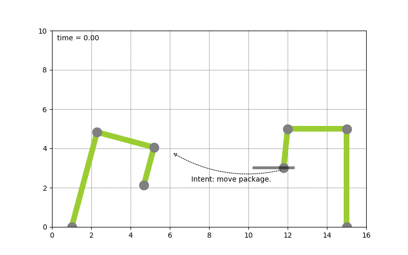
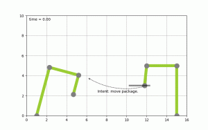
To make this more concrete I spend some time implementing planning algorithms to test concepts. Picture the following, let’s say you have two robot arms. And you just give the control system the goal to move a package from A to B you want the system to itself figure out how to move the arms, to pick the package up & move it from A to B. The following diagram shows this:
 (Click to enlarge & animate)
The goal of moving the package from A to B is converted into a plan by looking at the state of the packages which is given by it’s coordinates. By picking up the package and moving it around the state of the package hence changes. The movement of the robot arms is constraint, while the smallest part of the robot arm can move by 1 degree during each time step the bigger parts of the arm can move by 2 & 5 degrees respectively.
Based on this, a state graph can be generated. Where the nodes of the graph define the state of the package (it’s position) and the edges actions that can be performed to alter those states (e.g. move a part of an robot arm, pick & drop package etc.). Obviously not all actions would lead to an optimal solution so the weights on the edges also define how useful this action can be. On top of that, an heuristic can be used that allows the planning algorithm to find it’s goal faster. To figure out the steps needed to move the package from A to B, we need to search this state graph and the “lowest cost” path between start state (package is at location A) and end state (package is at location B) defines the plan (or the steps on what/how to achieve the goal). For the example above, I used D* Lite.
Now that a plan (or series of step) is known we can use traditional scheduling techniques to figure out in which order to perform these. Also note the handover of the package between the robots to move it from A to B this shows – especially in distributed systems – that coordination is key. More on that will follow in a next blog-post.
Categories: Personal • Tags: Algorithm, Artificial Intelligence, Autonomic System, Distributed Systems, Machine Learning, Planning • Permalink for this article
November 18th, 2017 • Comments Off on Q-Learning in python
There is a nice tutorial that explains how Q-Learning works here. The following python code implements the basic principals of Q-Learning:
Let’s assume we have a state matrix defining how we can transition between states, and a goal state (5):
GOAL_STATE = 5
# rows are states, columns are actions
STATE_MATRIX = np.array([[np.nan, np.nan, np.nan, np.nan, 0., np.nan],
                         [np.nan, np.nan, np.nan, 0., np.nan, 100.],
                         [np.nan, np.nan, np.nan, 0., np.nan, np.nan],
                         [np.nan, 0., 0., np.nan, 0., np.nan],
                         [0., np.nan, np.nan, 0, np.nan, 100.],
                         [np.nan, 0., np.nan, np.nan, 0, 100.]])
Q_MATRIX = np.zeros(STATE_MATRIX.shape)
Visually this can be represented as follows:

(Click to enlarge)
For example if you are in state 0, we can go to state 4, define by the 0. . If we are in state 4, we can directly goto to state 5 define by the 100. . np.nan define impossible transitions. Finally we initialize an empty Q-Matrix.
Now the Q-Learning algorithm is simple. The comments in the following code segment will guide through the steps:
i = 0
while i < MAX_EPISODES:
    # pick a random state
    state = random.randint(0, 5)
    while state != goal_state:
        # find possible actions for this state.
        candidate_actions = _find_next(STATE_MATRIX[state])

        # randomly pick one action.
        action = random.choice(candidate_actions)

        # determine what the next states could be for this action...
        next_actions = _find_next(STATE_MATRIX[action])
        values = []
        for item in next_actions:
            values.append(Q_MATRIX[action][item])

        # add some exploration randomness...
        if random.random() < EPSILON:
            # so we do not always select the best...
            max_val = random.choice(values)
        else:
            max_val = max(values)

        # calc the Q value matrix...
        Q_MATRIX[state][action] = STATE_MATRIX[state][action] + \
                                  EPSILON * max_val

        # next step.
        state = action
    i += 1
We need one little helper routine for this – it will help in determine the next possible step I can do:
def _find_next(items):
    res = []
    i = 0
    for item in items:
        if item >= 0:
            res.append(i)
        i += 1
    return res
Finally we can output the results:
Q_MATRIX = Q_MATRIX / Q_MATRIX.max()

np.set_printoptions(formatter={'float': '{: 0.3f}'.format})
print Q_MATRIX
This will output the following Q-Matrix:
[[ 0.000  0.000  0.000  0.000  0.800  0.000]
 [ 0.000  0.000  0.000  0.168  0.000  1.000]
 [ 0.000  0.000  0.000  0.107  0.000  0.000]
 [ 0.000  0.800  0.134  0.000  0.134  0.000]
 [ 0.044  0.000  0.000  0.107  0.000  1.000]
 [ 0.000  0.000  0.000  0.000  0.000  0.000]]
This details for example the best path to get from e.g. state 2 to state 5 is: 2 -> 3 (0.107), 3 -> 1 (0.8), 1 -> 5 (1.0).
Categories: Personal • Tags: Machine Learning, Python • Permalink for this article
July 25th, 2016 • Comments Off on Insight driven resource management & scheduling
Future data center resource and workload managers – and their [distributed]schedulers – will require a new key integrate capability: analytics. Reason for this is the the pure scale and the complexity of the disaggregation of resources and workloads which requires getting deeper insights to make better actuation decisions.
For data center management two major factors play a role: the workload (processes, tasks, containers, VMs, …) and the resources (CPUs, MEM, disks, power supplies, fans, …) under control. These form the service and resource landscape and are specific to the context of the individual data center. Different providers use different (heterogeneous) hardware (revisions) resource and have different customer groups running different workloads. The landscape overall describes how the entities in the data center are spatially connected. Telemetry systems allow for observing how they behave over time.
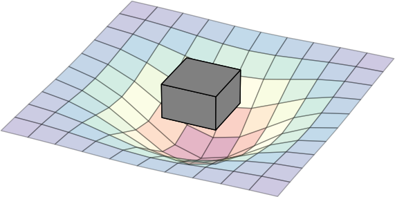
The following diagram can be seen as a metaphor on how the two interact: the workload create a impact on the landscape. The box represent a simple workload having an impact on the resource landscape. The landscape would be composed of all kind of different entities in the data center: from the air conditioning facility all the way to the CPU. Obviously the model taken here is very simple and in real-life a service would span multiple service components (such as load-balancers, DBs, frontends, backends, …). Different kinds of workloads impact the resource landscape in different ways.

(Click to enlarge)
Current data center management systems are too focused on understanding resources behavior only and while external analytics capabilities exists, it becomes crucial that these capabilities need to move to the core of it and allow for observing and deriving insights for both the workload and resource behavior:
- workload behavior: Methodologies such as described in this paper, become key to understand the (heterogeneous) workload behavior and it’s service life-cycle over space and time. This basically means learning the shape of the workload – think of it as the form and size of the tile in the game Tetris.
- resource behavior: It needs to be understood how a) heterogeneous workloads impact the resources (especially in the case of over-subscription) and b) how features of the resource can impact the workload performance. Think of the resources available as the playing field of the game Tetris. Concept as described in this paper help understand how features like SR-IOV impact workload performance, or how to better dimension the service component’s deployment.
Deriving insights on how workloads behave during the life-cycle, and how resources react to that impact, as well as how they can enhance the service delivery is ultimately key to finding the best match between service components over space and time. Better matching (aka actually playing Tetris – and smartly placing the title on the playing field) allows for optimized TCO given a certain business objective. Hence it is key that the analytical capabilities for getting insights on workload and resource behavior move to the very core of the workload and resource management systems in future to make better insightful decisions. This btw is key on all levels of the system hierarchy: on single resource, hosts, resource group and cluster level.
Note: parts of this were discussed during the 9th workshop on cloud control.
Categories: Personal • Tags: Analytics, Cloud, data center, Machine Learning, Orchestration, Scheduling, SDI • Permalink for this article
March 21st, 2016 • 1 Comment
Orchestration and Scheduling are not the newest topics, in fact they have been used in distributed systems forever (as in a couple of decades :-)). Systems like Mesos and Kubernetes (or offerings like Mantl) have brought advancements when it comes to dealing with scale. Other systems have a great background in scheduling and offer many (read a whole lot) policies for the same, this includes technologies like Grid Engine, LSF/OpenLava, etc.. Actually some of these technologies integrate with each other (like navops, Kubernetes and Mesos, OpenLava and Mesos, …), which makes it for example interesting when dealing with scheduling for space & order at the same time.
Next to pure demand, upcoming trends like CNCF & OCI as well as the introduction of Software Defined Infrastructure (SDI) drive the number of resources and services the Orchestrators and Controllers manage up. And the Question arises how to efficiently manage your data center – doing it by a human pressing a button is just not going to scale 🙂
Feedback control systems are a great start, however have some drawbacks. The larger the scale the more conflicts you might get between the feedback loops. The approaches might work up to rack level but probably not much beyond that. For large scale we need an approach which works along the lines of watch (e.g. by using snap), learn/decide (e.g. by using TAP) and act (See Jason Waxman’s keynote at OCP). This will eventually allow for a operatorless/humanless/driverless operations of the data center to support autonomous operations for scaling, healing and optimizing e.g. TCO.
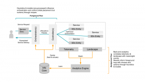
Within Intel Labs we have therefore come up with the concept of a foreground and a background flow. Within a continuously running background flow we observe (if needed over long time-periods) the data center with its resources and services and try to derive & update models heuristics (read: rule of thumb) continuously using analytics/machine learning. Within a foreground flow – which sometimes is denoted the fast loop as it needs to perform – we can than score against those heuristics/models in actions plans/recipes.
The action plan/recipes describe a process on how we deal with a initial placement or re-balancing event. The scoring will allow for making better initial placement (adding a workload) as well as re-balancing decisions (how/what/when to kill, migrate or tune the infrastructure). How to derive an heuristics is explained in a paper referenced below – the example within that is about to learn how to best place a VNF so that is makes optimal use of platform features such as SR-IOV. Multiple other heuristics can easily be imagined, like learning how many cores a certain workload needs.
The following diagram shows the background and foreground flow.
(Click to enlarge)
The heuristics are stored in an Information Core which based on the environment it is deployed in tunes itself. We’ve defined the concepts described here in a paper submitted to the Middleware 2015 conference. The researchers from Umea (who also run this highly recommended workshop) have used it and demonstrate an example use case in the same paper. For an example on how a background flow can help informing the foreground flow read this short paper. (Excuses for the paywall :-))
I’ll follow-up with some more blog posts detailing certain aspects of our latest work/research, like how the landscape works.
Categories: Work • Tags: Analytics, Cloud, data center, Machine Learning, Orchestration, Scheduling, SDI • Permalink for this article
October 30th, 2014 • Comments Off on American Football Game Analysis
I’ve been coaching American Football for a while now and it is a blast standing on the sideline during game day. The not so “funny” part of coaching however – especially as Defense Coordinator – is the endless hours spend on making up stats of the offensive strategy of the opponent. Time to save some time and let the computer do the work.
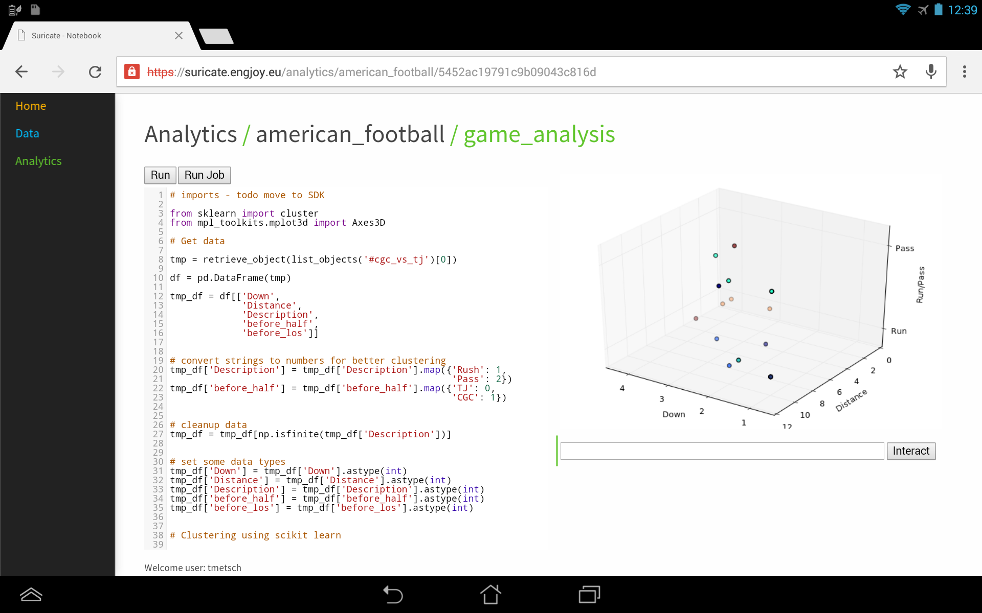
I’ve posted about how you could use suricate in a sports data setup past. The following screen shot show the first baby steps (On purpose not the latest and greatest – sry 🙂 ) of analyzing game data using suricate with python pandas and scikit-learn for some clustering. The 3D plot shows Down & Distance vs Run/Pass plays. This is just raw data coming from e.g. here.
The colors of the dots actually have a meaning in such that they represent a clustering of many past plays. The clustering is done not only on Down & Distance but also on factors like field position etc. So a cluster can be seen as a group of plays with similar characteristics for now. These clusters can later be used to identify a upcoming play which is in a similar cluster.
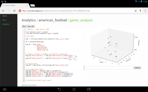
(Click to enlarge)
The output of this python script stores processed data back to the object store of suricate.
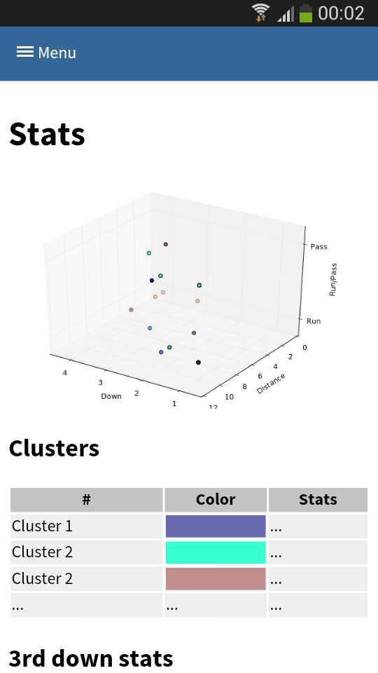
One of the new features of suricate is template-able dashboards (not shown in past screenshot). Which basically means you can create custom dashboards with fancy graphics (choose you poison: D3, matplotlib, etc):

(Click to enlarge)
Again some data is left out for simplicity & secrecy 🙂
Making use of the stats
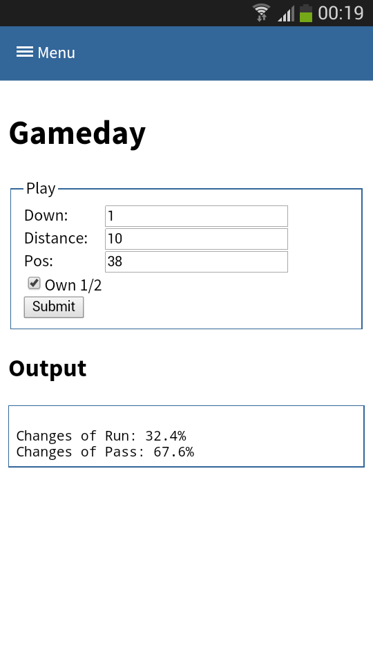
One part is understanding the stats as created in the first part. Secondly acting upon it is more important. With Tablets taking on sidelines, it is time to do the same & take the stats with you on game day. I have a simple web app sitting around in which current ball position is entered and some basic stats are shown.
This little web application does two things:
- Send a AMQP msg with the last play information to a RabbitMQ broker. Based on this new message new stats are calculated and stored back to the game data. This works thanks to suricate’s streaming support.
- Trigger suricate to re-calculate the changes of Run-vs-Pass in an upcoming play.
The webapp is a simple WSGI python application – still the hard work is carried out by suricate. Nevertheless the screenshot below shows the basic concept:

(Click to enlarge)
Categories: Personal, Sports • Tags: American Football, Data Science, Machine Learning, Python • Permalink for this article