October 15th, 2013 • 2 Comments
With this blog post I try to summarize some key concepts/definitions of something called an Analytics-as-a-Service (AaaS). The AaaS – named Suricate – described in this post , was developed as part of my Masterthesis. The Masterthesis was about learning application/service behavior and then be able to abstract models from that, to create agile systems/strategies. This could reach from simple fault-detection up to reconfigurations (e.g. auto scaling) of the application/service instance of the platform (Cloud/whatever) it runs upon. Originally it was used to take data aggregated from DTrace using Python, parse models from it using scikit-learn, continuously compare (and update) models with new incoming data, and finally process/take actions. This process requires sometimes user interactions (from Data Scientist or whatever you wanna call them) as can be seen in the following diagram:
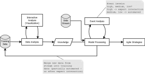
Learning Process (Click to enlarge)
Eventually, when my Masterthesis was done (with much more in it then just the development of Suricate in it – talking algorithms/concepts to create models etc), I thought it could serve some more general purpose. In short (tl;dr 🙂) Suricate:
- allows you to upload or stream data so the Service can aggregate it.
- allows a Data Scientist to perform Analytics and visualize the results.
- supports the processing and acting (trigger actions) on the analysis and thereby the creation of continuously adjusted agile Systems & Strategies based on up-to-date insights.
Concepts of an Analytics as a Service
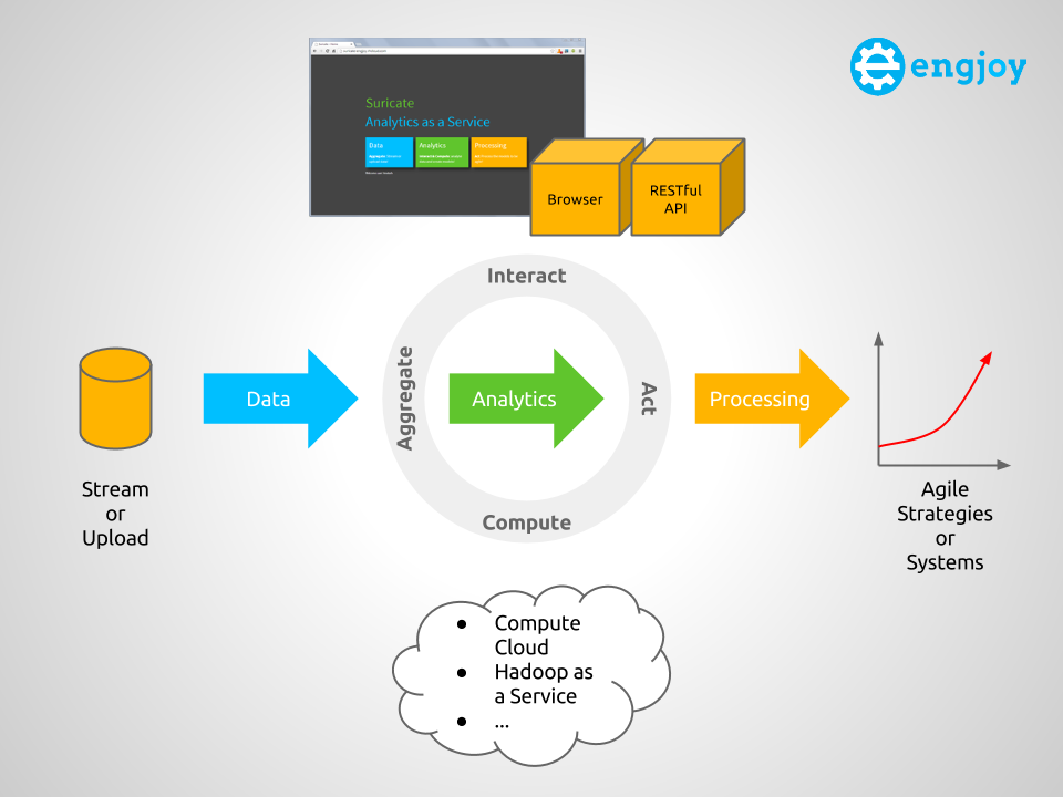
The following diagram shows a conceptual overview of Suricate, which will be used to explain some key concepts of an AaaS.

Overview of Suricate – Analytics as a Service (Click to enlarge)
Overall the four main concepts for an AaaS therefore are:
- Aggregate – Supplying user defined data: Stream data into the service or upload the data in an internal or external Storage (Object, Relational, etc). The data can then be aggregated, pre-processed and cached.
- Interact – Supplying user defined logic (this is where the IP is in – create marketplace for this if you want :-)): Use Python interactive scripting capabilities to perform analytics and visualize (visualizations are sometimes key to understanding :-)) the results. The Data Scientist can interact with the Service via a Web UI or REST API.
- Compute – Uses other services (potentially compute or things like Hadoop) to perform the computational aspect of the analytics.
- Act – Process the learned models and trigger actions on insights gained, to create agile Systems & Strategies.
Other example of AaaS are Quantopian or DataHero btw. There are plenty of other around, but most of them are focused on Business Analytics. But sometimes the streaming data & ‘Acting’ part is missing from all of them. When running Suricate one is first greeted with the overview page. Those ’tiles’ reflecting the main concepts of an AaaS:
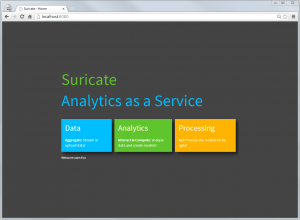
Suricate entry (Click to enlarge)
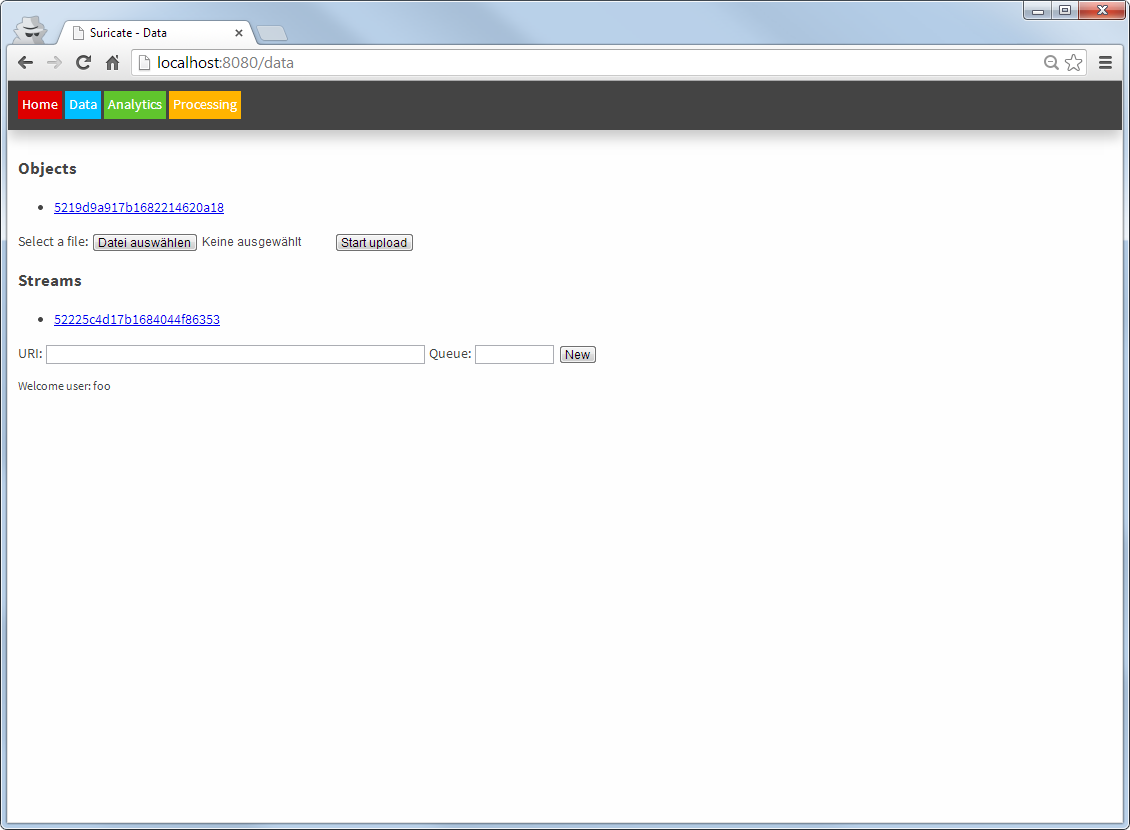
In the data page, files can be uploaded as objects and AMQP streams can be defined:

Suricate data sources (Click to enlarge)
In the Analytics part notebooks – just like with IPython – can be written. Within these notebooks toolkits such as matplotlib, scikit-learn or Python Pandas can easily be used. Using these toolkits models can be created within this part and stored again as objects (or even use them to retrieve/download data from somewhere). Also packages to enable faster computation of models can be integrated, as a full Python interpreter is at hands. Python is an ideal language for data processing/analytics and learning btw [1], [2] – although R could be integrated too.
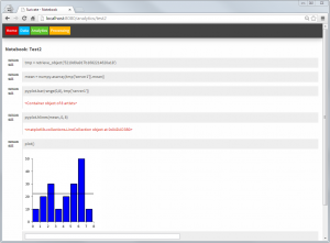
Suricate Analytics – model creation (Click to enlarge)
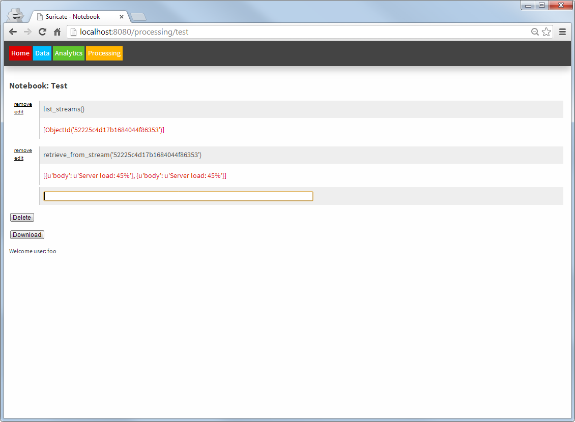
The Processing part looks similar to the Analytics part. Again notebooks can be created. But these notebooks now use the models created earlier, to compare them with new incoming data (from AMQP) streams and take actions accordingly.

Suricate processing (Click to enlarge)
It is noted here that both the processing and the Analytics notebooks can be triggered externally (through an API), and therefore create a true continuously Analytics framework.
Suricate’s source code is available (without warranty – Open Source – in early stages etc. as it is mainly a Demonstrator/PoC for my thesis) on GitHub. Feel free to extent it etc. It happily runs on PaaS like OpenShift as it is an simple WSGI application.
Categories: Personal • Tags: Analytics, Data Science, DTrace, Machine Learning, Python • Permalink for this article
July 16th, 2013 • Comments Off on Learn Service Behaviour
This started off as just an idea in my head a while ago and soon become my Master thesis. The idea is to apply Machine Learning/Data Analysis methodologies to Data derived from tools such as DTrace. Based on the learned knowledge it would then be possible to create adaptive/agile systems. For example to balance out your workload as a service provider overnight. Or move your compute close to your data. Or to learn how to best configure your system (by using Software Defined Networking). Or to simple tune your threshold values in your monitoring system etc. Or you name it – it might be doable.
After finally finishing my Master thesis – doing that next to work is quite a challenge I can tell now 🙂 – I can certainly say that some stuff can indeed be learned. During the work on my thesis I sketched out a, in browser programmable (Python of course :-)), Analytics as a Service (I just like the acronym for it :-)) which can be used learn from Data derived from DTrace (See 1).
As a first step it is useful to select the resources you want to look at. The should have a relevance to the behavior of the applications and services. The USE Method demoed by Brendan Gregg might be a good start. Once you know what you want to look for it is possible to gather some data. For example using the DTrace consumer for Python (See 2), like I did. Cool think is now that thanks to Python you can send it around (pika), store it (MongoDB, sqlite) and process it (scikit-learn) easily. Just add a few API for abstraction, a rich web application for creating python notebooks and you have the Analytics as a Service.
Now we can work through the data with some simple steps.
- Step 1 – Analyze the time series you got with some first methods. This could reach from calculating means, averages, etc over smoothing or regression analyses to looking into correlations in the data. Now you will have a good knowledge of which time series are interesting for further analysis.
- Step 2 – Cluster the applications/services based on the data points to get an first overview of how they fit together. Again simple k-means clustering can be an initial step. Remember sometimes the simplest methods are the best 🙂
- Step 3 – Based on what has been learned till now try to apply mechanism to analyze the covariance/correlation between the applications/services. Once done you get a nice graph which represents behavior of your overall environment.
- Step 4 – Go beyond the simple and try to build Bayesian networks on what you got now. Go look at decision trees if possible to try build that adaptive/agile system.
- Step 5 – Well as usual the sky might actually be the limit.
Results of each of the steps can be seen as models which can be compared with new incoming data from DTrace. Based on the ‘intelligence’ of the comparison of the new date with the learn model (knowledge) the adaptive/agile system can be build. Continuously updating your learned model in the learning process is key – we don’t want to ‘predict’ the future using a crystal ball. This is just the tip of the iceberg of all stuff worked on and discovered in my Master thesis – but as usual – so little time so much to do 🙂 But maybe I’ll find some time soon to sketch out the learning process and share some details of what I was able to let the computer learn…
Categories: Personal • Tags: Analytics, Data Science, DTrace, Machine Learning, OpenSolaris, Python, SmartOS • Permalink for this article
March 24th, 2013 • Comments Off on Learning application behavior
I have been working for a while now on bringing together some very interesting topics. Machine learning/data analysis tools and the platform I like: SmartOS with it’s great DTrace tooling. This is a first post on this topics with some very early results 🙂
The following graph shows the dependencies between some processes (got way more in my dataset). The ones with ‘*_tracer‘ run within a zone. Whereas the ‘*_platform‘ are coming from the global SmartOS zone. To make it more complete also I/O of the platform are taken into account, so we do not just look at the processes. The graph shows the ‘links’ between the processes (e.g. python) & other data sources (iops):

Inter-dependencies of proccesses
What happened within the time-frame of the training data was that another zone with an KVM VM instances got started, hence the ‘qemu‘ process running. First a cluster analysis was used to see the rough interdependence of the sources. The edges express the ‘strength’ of an link between data sources – this was inspired by this.
You can see that the start of a VM leads to some I/O operations, logically. The python process you can see has a strong link to the qemu process for no particular reason. This is because it was collecting data using the DTrace consumer. So it just happens that is was very active while the KVM got started. As said this is a first shot. Certainly the selection to which data sources to look at needs to be optimized. Plenty of possibilities there since I used DTrace to gather a fair amount of data.
Also it will be interesting to look at different application setups. This was data gathered during a VM start up. First experiments while looking at web severs (the httpd process and incoming tcp connections) already bring up different graphs. So why is this cool? When an machine can learn the behavior (graphs like above) it can identify misbehavior based on new incoming data from a DTrace probes. Also this could be used to tune the setup & configurations of a system.
Again these are very early results – just got excited and wanted to post something 🙂 Definitely the cluster analysis which is carried out needs to be tuned as well.
What was used to get this done:
And just for fun since I discovered this nice XKCD plotting extension to matplotlib – a graph which show the # of system calls per process over time in xkcd ‘style’:

System calls per process over time
Categories: Personal • Tags: Analytics, DTrace, Machine Learning, Python, SmartOS • Permalink for this article
May 20th, 2012 • 3 Comments
In previous blogposts I already demoed what a Python based DTrace consumer can be used for: live inspection (callgraphs) of running programs, nice Visualizations or just plain tracing. Especially with SmartOS (as one of the many platforms which have DTrace support)I found it a bit annoying to deal with DTrace. Since SmartOS is headless itself I was thinking about creating a web based editor for DTrace scripts which would than create nice visualizations of the aggregated data. This simple IDE is written as an Django application and makes use of the Python based DTrace consumer.
So here it is a first shot of the DTrace web based Mini-IDE (couldn’t come up with a better name :-))

web based DTrace IDE (Click to enlarge)
As you can see it is running inside of Chrome on a Windows box – just to make sure you believe it is indeed web based. Now let’s take a look at all the features:
Syntax highlighting & Error detection
The user is guide through 3 steps – Writing the DTrace script, running it and then the output is shown. The editor in the first step features a DTrace specific syntax highlighting. Variables, Build-in variables, functions, aggregation functions and a set of providers are highlighted accordingly. Comments are also parsed in a certain color.
Next to this the editor will try to compile the script and show possible errors. The following screen-shot shows that when an unknown aggregation function is used the error is reported. It will use the Python binding for libdtrace to compile the script and return any errors:

Wrong aggregation function name (Click to enlarge)
Running DTrace
When clicking next to reach the next step a set of options are shown. The user can insert the time in seconds which DTrace should aggregate data (In this case 2 – or 0 when continuously aggregate data) and check if a chart should be generated from the aggregated data:

Options for running DTrace (Click to enlarge)
Displaying the result
When done the aggregated Data will be displayed. E.g. when you used the following one liner (syscall count by syscall):
syscall:::entry {
    @num[probefunc] = count();
}
The result is displayed as a pie chart:

(Click to enlarge)
Or to give another example (A read distribution):
syscall::read:entry {
    @dist[execname] = lquantize(arg0, 0, 12, 2);
}
The result would be a bit different since the aggregation function lquantize is used. The data is displayed from 0 to 12 in steps of 2. The Z-Axis shows the name of the executable:

(Click to enlarge)
Categories: Personal • Tags: Analytics, DTrace, Python • Permalink for this article
April 1st, 2012 • Comments Off on Python DTrace consumer and AMQP
This blog post will lead through an very simple example to show how you can use the Python DTrace consumer and AMQP.
The scenario for this example is pretty simple – let’s say you want to trace data on one machine and display it on another. Still the data should be up to date – so basically whenever a DTrace probe fires the data should be transmitted to the other hosts. This can be done with AMQP.
The examples here assume you have a RabbitMQ server running and have pika installed.
Within this example two Python scripts are involved. One for sending data (send.py) and one for receiving (receive.py). The send.py script will launch the DTrace consumer and gather data for 5 seconds:
thr = dtrace.DTraceConsumerThread(SCRIPT, walk_func=walk)
thr.start()
time.sleep(5)
thr.stop()
thr.join()
The DTrace consumer is given an callback function which will be called whenever the DTrace probes fire. Within this callback we are going to create a message ad pass it on to the AMQP broker:
def walk(id, key, value):
    channel.basic_publish(exchange='', routing_key='dtrace', body=str({key[0]: value}))
The channel has previously been initialized (See this tutorial on more details). Now AMQP messages are passed around with up-to-date information from DTrace. All that there is left is implementing a ‘receiver’ in receive.py. This is again straight forward and also works using a callback function:
def callback(ch, method, properties, body):
    print 'Received: ', data

if __name__ == '__main__':
    channel.basic_consume(callback, queue='dtrace', no_ack=True)
    try:
        channel.start_consuming()
    except KeyboardInterrupt:
        connection.close()
Start the receive.py Python script first. Than start the send.py Python script. You can even start multiple send.py scripts on multiple hosts to get an overall view of the system calls made by processes on all machines 🙂
The send.py script counts system calls and will send AMQP messages as new data arrives. You will see in the output of the receive.py script that data arrives almost instantly:
$ ./receive.py
Received:  python 264
Received:  wnck-applet 5
Received:  metacity 6
Received:  gnome-panel 15
[...]
Now you can build life updating visualizations of the data gathered by DTrace.
Categories: Personal • Tags: Analytics, DTrace, Python • Permalink for this article