No Huddle Offense

American Football Game Analysis

I’ve been coaching American Football for a while now and it is a blast standing on the sideline during game day. The not so “funny” part of coaching however – especially as Defense Coordinator – is the endless hours spend on making up stats of the offensive strategy of the opponent. Time to save some time and let the computer do the work.

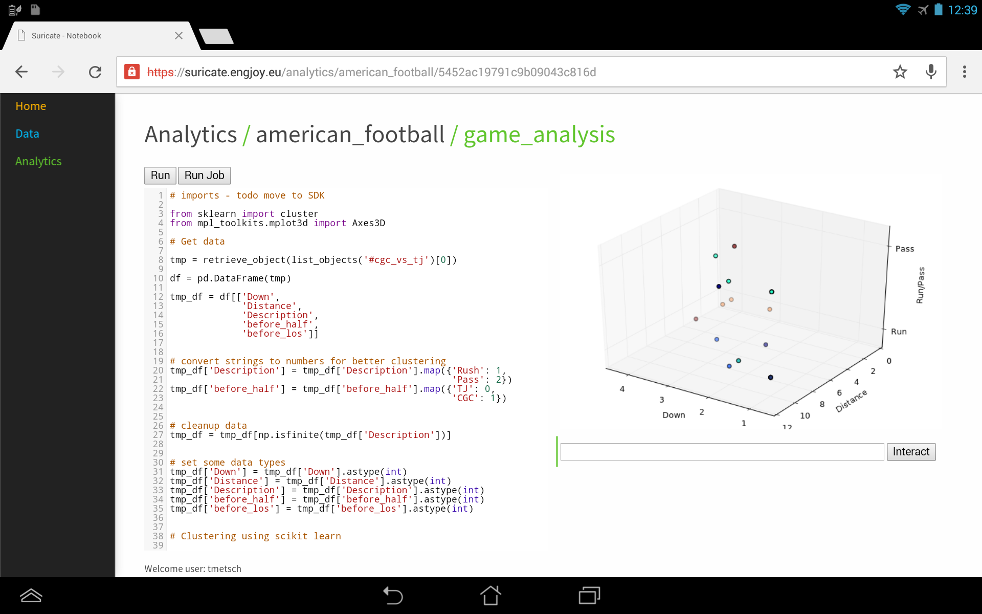
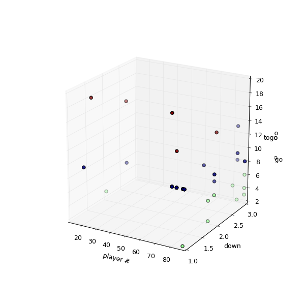
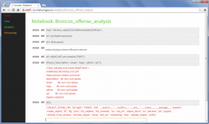
I’ve posted about how you could use suricate in a sports data setup past. The following screen shot show the first baby steps (On purpose not the latest and greatest – sry 🙂 ) of analyzing game data using suricate with python pandas and scikit-learn for some clustering. The 3D plot shows Down & Distance vs Run/Pass plays. This is just raw data coming from e.g. here.

The colors of the dots actually have a meaning in such that they represent a clustering of many past plays. The clustering is done not only on Down & Distance but also on factors like field position etc. So a cluster can be seen as a group of plays with similar characteristics for now. These clusters can later be used to identify a upcoming play which is in a similar cluster.

(Click to enlarge)

The output of this python script stores processed data back to the object store of suricate.

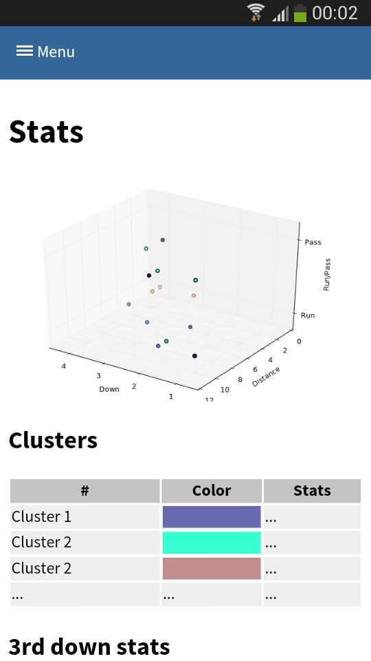
One of the new features of suricate is template-able dashboards (not shown in past screenshot). Which basically means you can create custom dashboards with fancy graphics (choose you poison: D3, matplotlib, etc):

(Click to enlarge)

Again some data is left out for simplicity & secrecy 🙂

Making use of the stats

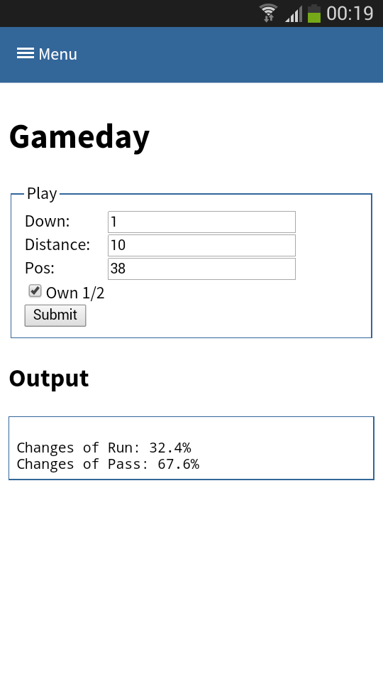
One part is understanding the stats as created in the first part. Secondly acting upon it is more important. With Tablets taking on sidelines, it is time to do the same & take the stats with you on game day. I have a simple web app sitting around in which current ball position is entered and some basic stats are shown.

This little web application does two things:

1. Send a AMQP msg with the last play information to a RabbitMQ broker. Based on this new message new stats are calculated and stored back to the game data. This works thanks to suricate’s streaming support.
2. Trigger suricate to re-calculate the changes of Run-vs-Pass in an upcoming play.

The webapp is a simple WSGI python application – still the hard work is carried out by suricate. Nevertheless the screenshot below shows the basic concept:

(Click to enlarge)

Categories: Personal, Sports • Tags: American Football, Data Science, Machine Learning, Python • Permalink for this article

Running a distributed native-cloud python app on a CoreOS cluster

Suricate is an open source Data Science platform. As it is architected to be a native-cloud app, it is composed into multiple parts:

• a web frontend (which can be load-balanced)
• execution nodes which actually perform the data science tasks for the user (for now each user must have at least one exec node assigned)
• a mongo database for storage (which can be clustered for HA)
• a RabbitMQ messaging system  (which can be clustered for HA)

Up till now each part was running in a SmartOS zone in my test setup or run with Openhift Gears. But I wanted to give CoreOS a shot and slowly get into using things like Kubernetes. This tutorial hence will guide through creating: the Docker image needed, the deployment of RabbitMQ & MongoDB as well as deployment of the services of Suricate itself on top of a CoreOS cluster. We’ll use suricate as an example case here – it is also the general instructions to running distributed python apps on CoreOS.

Step 0) Get a CoreOS cluster up & running

Best done using VagrantUp and this repository.

Step 1) Creating a docker image with the python app embedded

Initially we need to create a docker image which embeds the Python application itself. Therefore we will create a image based on Ubuntu and install the necessary requirements. To get started create a new directory – within initialize a git repository. Once done we’ll embed the python code we want to run using a git submodule.

$ git init
$ git submodule add https://github.com/engjoy/suricate.git

Now we’ll create a little directory called misc and dump the python scripts in it which execute the frontend and execution node of suricate. The requirements.txt file is a pip requirements file.

 
$ ls -ltr misc/
total 12
-rw-r--r-- 1 core core 20 Sep 21 11:53 requirements.txt
-rw-r--r-- 1 core core 737 Sep 21 12:21 frontend.py
-rw-r--r-- 1 core core 764 Sep 21 12:29 execnode.py 

Now it is down to creating a Dockerfile which will install the requirements and make sure the suricate application is deployed:

 
$ cat Dockerfile
FROM ubuntu
MAINTAINER engjoy UG (haftungsbeschraenkt)

# apt-get stuff
RUN echo "deb http://archive.ubuntu.com/ubuntu/ trusty main universe" >> /etc/apt/sources.list
RUN apt-get update
RUN apt-get install -y tar build-essential
RUN apt-get install -y python python-dev python-distribute python-pip

# deploy suricate
ADD /misc /misc
ADD /suricate /suricate

RUN pip install -r /misc/requirements.txt

RUN cd suricate && python setup.py install && cd ..

Now all there is left to do is to build the image:

 
$ docker build -t docker/suricate .

Now we have a docker image we can use for both the frontend and execution nodes of suricate. When starting the docker container we will just make sure to start the right executable.

Note.: Once done publish all on DockerHub – that’ll make live easy for you in future.

Step 2) Getting RabbitMQ and MongoDB up & running as units

Before getting suricate up and running we need a RabbitMq broker and a Mongo database. These are just dependencies for our app – your app might need a different set of services. Download the docker images first:

 
$ docker pull tutum/rabbitmq
$ docker pull dockerfile/mongodb

Now we will need to define the RabbitMQ service as a CoreOS unit in a file call rabbitmq.service:

 
$ cat rabbitmq.service
[Unit]
Description=RabbitMQ server
After=docker.service
Requires=docker.service
After=etcd.service
Requires=etcd.service

[Service]
ExecStartPre=/bin/sh -c "/usr/bin/docker rm -f rabbitmq > /dev/null ; true"
ExecStart=/usr/bin/docker run -p 5672:5672 -p 15672:15672 -e RABBITMQ_PASS=secret --name rabbitmq tutum/rabbitmq
ExecStop=/usr/bin/docker stop rabbitmq
ExecStopPost=/usr/bin/docker rm -f rabbitmq

Now in CoreOS we can use fleet to start the rabbitmq service:

 
$ fleetctl start rabbitmq.service
$ fleetctl list-units
UNIT                    MACHINE                         ACTIVE  SUB
rabbitmq.service        b9239746.../172.17.8.101        active  running

The CoreOS cluster will make sure the docker container is launched and RabbitMQ is up & running. More on fleet & scheduling can be found here.

This steps needs to be repeated for the MongoDB service. But afterall it is just a change of the Exec* scripts above (Mind the port setups!). Once done MongoDB and RabbitMQ will happily run:

 
$ fleetctl list-units
UNIT                    MACHINE                         ACTIVE  SUB
mongo.service           b9239746.../172.17.8.101        active  running
rabbitmq.service        b9239746.../172.17.8.101        active  running

Step 3) Run frontend and execution nodes of suricate.

Now it is time to bring up the python application. As we have defined a docker image called engjoy/suricate in step 1 we just need to define the units for CoreOS fleet again. For the frontend we create:

 
$ cat frontend.service
[Unit]
Description=Exec node server
After=docker.service
Requires=docker.service
After=etcd.service
Requires=etcd.service

[Service]
ExecStartPre=/bin/sh -c "/usr/bin/docker rm -f suricate > /dev/null ; true"
ExecStart=/usr/bin/docker run -p 8888:8888 --name suricate -e MONGO_URI=<change uri> -e RABBITMQ_URI=<change uri> engjoy/suricate python /misc/frontend.py
ExecStop=/usr/bin/docker stop suricate
ExecStopPost=/usr/bin/docker rm -f suricate

As you can see it will use the engjoy/suricate image from above and just run the python command. The frontend is now up & running. The same steps need to be repeated for the execution node. As we run at least one execution node per tenant we’ll get multiple units for now. After bringing up multiple execution nodes and the frontend the list of units looks like:

 
$ fleetctl list-units
UNIT                    MACHINE                         ACTIVE  SUB
exec_node_user1.service b9239746.../172.17.8.101        active  running
exec_node_user2.service b9239746.../172.17.8.101        active  running
frontend.service        b9239746.../172.17.8.101        active  running
mongo.service           b9239746.../172.17.8.101        active  running
rabbitmq.service        b9239746.../172.17.8.101        active  running
[...]

Now your distributed Python app is happily running on a CoreOS cluster.

Some notes

• Container building can be repeated without the need to destroy: docker build -t engjoy/suricate .
• Getting the log output of container to check why the python app crashed: docker logs <container name>
• Sometimes it is handy to test the docker run command before defining the unit files in CoreOS
• Mongo storage should be shared – do this by adding the following to the docker run command: -v <db-dir>:/data/db
• fleetctl destroy <unit> and list-units are you’re friends 🙂
• The files above with simplified scheduling & authentication examples can be found here.

Categories: Personal • Tags: Analytics, Cloud, CoreOS, Data Science, Python, Software Engineering, Tech • Permalink for this article

Live football game analysis

Note: I’m talking about American Football here 🙂

In previous posts I already showed how game statistics can be used to automatically which Wide receiver is the Qb’s favorite on which play, down and field position. Now let’s take this one step further and create a little system (using Suricate) which will make suggestions to a Defense Coordinator.

The following diagram will guide through the steps needed to create such a system:

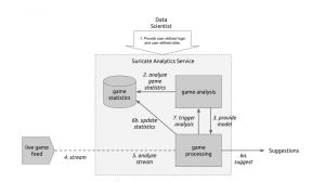
Live game breakdown (Click to enlarge)

Let’s start at the top. (Step 1) The User of Suricate will start with performing some simple steps. First a bunch of game statistics are uploaded (same as using in this post). Next also a stream is defined. In this case a URI for an AMQP broker (using CloudAMQP – RabbitMQ as a Service) is defined in the service. With this used defined data is provide to the service.

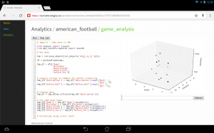
(Step 2) Now we start creating an analytics notebook. Suricate provides an interactive python console via your web browser which can easily be used to explore the data previously uploaded. Python Pandas and scikit-learn are both available within the Suricate service and can be used right away to accomplish this task:

Exploring game statistics (Click to enlarge)

Based on the data we can create a model which describes on which down, on which fieldposition a run or a pass play is performed. We can also store who is the favorite Wide receiver/Running back for those plays (see also). All this information is stored in a JSON data structure and saved using the SDK of Suricate (Step 3).

(Step 4) Now a little external python script needs to be written which grabs relatively ‘live’ game data from e.g. here. This script now simple continuously sends messages to the previously defined RabbitMQ broker. The messages contain the current play, fieldposition and distance togo information.

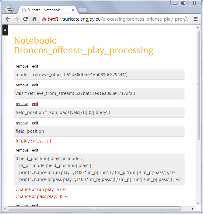
(Step 5) Now a processing python notebook needs to be written. This is a rather simple python script. It takes the new incoming messages and compares them to the model learned in step 2 & 3. Based on that suggestions can be displayed (Step 6a) – “e.g. watch out for Wes Welker on 3rd and long at own 20y line” or just some percentages for pass or run plays:

Processing notebook (Click to enlarge)

Next the information about the new play can be added to the game statics data file (Step 6b). Once this is done a new model can be created (Step 7) to get the most up to date models all the time.

With this overall system new incoming data is streamed in (continuous analytics), models updated and suggestions for a Defense Coordinator outputted. Disclaimer: some steps describe here are not yet in the github repository of suricate – most namely the continuously running of scripts.

Categories: Personal, Sports • Tags: American Football, Analytics, Data Science, Machine Learning • Permalink for this article

Peyton’s favorite WO (Analytics-as-a-Service)

Again a little excerpt on stuff you can do with the help of Suricate. Again we’ll look at play-by-play statistics. So no information on which play was performed, but just the outcomes of the plays. Still there is some information you can retrieve from that. Most importantly because it can be done automated without user interaction needed. Just upload the file, press a button and get the results:

Peyton’s favorites (Click to enlarge)

This time you are looking are a cluster analysis of players Peyton passed too in the game of week 1. First cluster represent players passed to on 1,2 & 3 down with up to 6 yards. The second cluster the goto-guys which did go for medium yardage and finally the WOs able to get a bunch of yards on the board.

So with simple scripts (few lines of code – which can be reused) it is possible to abstract information from just play-to-play statistics. I guess mostly important to Defense Coordinators who would love to get some information on the fly with the press of a button 🙂

Categories: Personal, Sports • Tags: American Football, Analytics, Data Science, Machine Learning, Python • Permalink for this article

Peyton’s favorite WR in week 1 (Analytics-as-a-Service)

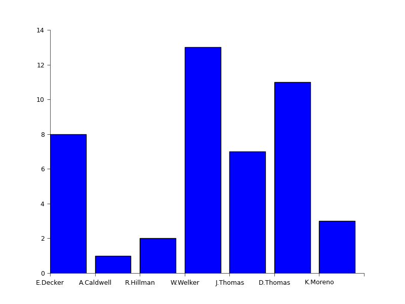
A few line lines of Python code, a big CSV file, some help of Python Pandas, Suricate and about 20 minutes is all it takes to answer the following Question:

Who was Peyton Manning’s favorite receiver during the match-up between Denver and Baltimore in week 1 of the 2013 NFL season?

The answer is simple: Wes Welker 🙂 See the complete graph below…

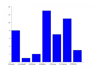
Peyton’s favorite (Click to enlarge)

Now it would be cool to find a source to stream the data into Suricate (which supports this) and get live up to date charts…but that is for another day.

Categories: Personal, Sports • Tags: American Football, Analytics, Data Science, Python • Permalink for this article