January 20th, 2019 • Comments Off on Dancing links, algorithm X and the n-queens puzzle
Donald Knuth’s 24th annual Christmas lecture inspired me to implement algorithm X using dancing links myself. To demonstrate how this algorithms works, I choose the n-queens puzzle. This problem has some interesting aspects to it which show all kinds of facets of the algorithm.
Solving the n-queens puzzle using algorithm X can be achieved as follows. Each queen being placed on a chess board will lead to 4 constraints that need to be cared for:
- There can only be one queen in the given row.
- There can only be one queen in the given column.
- There can only be one queen in the diagonal going from top left to bottom right.
- There can only be one queen in the diagonal going from bottom left to top right.
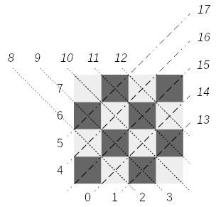
Let’s look at a chess board and determine some identifiers for each constraint that any placement can have (See the youtube video of the lecture at this timestep). Donald Knuth doesn’t go into too many details on how to solve this but let’s look at an 4×4 chessboard example:
 (Click to enlarge)
Assigning an identifier can be done straight forward: column based constraints are numbered 0-3; row based constraints get the ids from 4-7; diagonals 8-12; reverse diagonals 13-17 for a chessboard of size 4. Note that you can ignore the diagonal of size 1, as they are automatically covered by the row or column the queen would be placed in.
Calculating the identifiers for the constraints is simple. Given an queen positioned at coordinates (x, y) on a chessboard of size N these are the formulations you can use:
- the row constraint equals x
- the column constraint equals y + N
- for the diagonal constraint equals x + y + (2N-1)
- for the reverse diagonal constraint equals (N – 1 – x + y) + (4N-4)
Note that each constraint identifier calculation we use an offset, so we can all represent them in one context: 0 for the row constraints, N for the column constraints, 2N-1 for the diagonal and 4N-4 for the reverse diagonal constraints. For the diagonal constraints you need to ensure they are within their ranges: 2*N-1 < constraint < 3*N and 3*N+1 < constraint < 4*N + 1. If the calculated identifier of the constraints is not within the ranges, you can just drop the constraint – this is the case for queens being placed at corner positions. Placing a queen at coordinates (0,0) will result in 3 constraints: [0, 4, 15]. Placing a queen at coordinates (1,2) will results in 4 constraints: [1, 6, 10, 16].
Now that for each queen that can be placed we can calculate the uniquely identifiable constraints identifier, we can translate this problem into an exact cover problem. We are looking for a set of placed queens, for which all constraints can be satisfied. Let’s look at a matrix representation (for a chessboard of size 4, in which the rows are individual possible placements options of a queen, while the columns represent the constraints. The 1s indicate that it is a constraint that needs to be satisfied for the given placement.
| Queen coordinates | Primary constraints | Secondary constraints |
| x-coord | y-coord | diagonals | r-diagonals |
| 0 | 1 | 2 | 3 | 4 | 5 | 6 | 7 | 8 | 9 | 10 | 11 | 12 | 13 | 14 | 15 | 16 | 17 |
| 0,0 | 1 | | | | 1 | | | | | | | | | | | 1 | | |
| 0,1 | 1 | | | | | 1 | | | 1 | | | | | | | | 1 | |
| 0,2 | 1 | | | | | | 1 | | | 1 | | | | | | | | 1 |
| 0,3 | 1 | | | | | | | 1 | | | 1 | | | | | | | |
1,0
| | 1 | | | 1 | | | | 1 | | | | | | 1 | | | |
| 1,1 | | 1 | | | | 1 | | | | 1 | | | | | | 1 | | |
| 1,2 | | 1 | | | | | 1 | | | | 1 | | | | | | 1 | |
| 1,3 | | 1 | | | | | | 1 | | | | 1 | | | | | | 1 |
| 2,0 | | | 1 | | 1 | | | | | 1 | | | | 1 | | | | |
| 2,1 | | | 1 | | | 1 | | | | | 1 | | | | 1 | | | |
| 2,2 | | | 1 | | | | 1 |
| | | | 1 | | | | 1 | | |
| 2,3 | | | 1 | |
| | | 1 | | | | | 1 | | | | 1 | |
| 3,0 | | | | 1 | 1 |
| | | | | 1 | | | | | | | 1 |
| 3,1 | | | | 1 | | 1 |
| | | | | 1 | | 1 | | | | |
| 3,2 | | | | 1 | | | 1 | | | | | | 1 | | 1 | | | |
| 3,3 | | | | 1 | | | | 1 | | | | | | | | 1 | | |
Note that the table columns have been grouped into two categories: primary and secondary constraints. This is also a lesser known aspect of the algorithms at hand – primary columns and their constraints must be covered exactly once, while the secondary columns must only be covered at most once. Looking at the n-queens puzzle, this make sense – to fill the chessboard to the maximum possible number of queens, each row and column should have a queen, while there might be diagonals which are not blocked by a queen.
Implementing algorithm x using dancing links is reasonable simple – just follow the instructions in Knuth’s paper here. Let’s start with some Go code for the data structures:
type x struct {
	left  *x
	right *x
	up    *x
	down  *x
	col   *column
	data  string
}

type column struct {
	x
	size int
	name string
}

type Matrix struct {
	head      *x
	headers   []column
	solutions []*x
}
Note the little change I made to store a data string in the object x structure. This will be useful when printing the solutions later on. The following function in the can be used to initialize a new matrix:
func NewMatrix(n_primary, n_secondary int) *Matrix {
	n_cols := n_primary + n_secondary

	matrix := &Matrix{}
	matrix.headers = make([]column, n_cols)
	matrix.solutions = make([]*x, 0, 0)
	matrix.head = &x{}
	matrix.head.left = &matrix.headers[n_primary-1].x
	matrix.head.left.right = matrix.head

	prev := matrix.head
	for i := 0; i < n_cols; i++ {
		column := &matrix.headers[i]
		column.col = column
		column.up = &column.x
		column.down = &column.x
		if i < n_primary {
			// these are must have constraints.
			column.left = prev
			prev.right = &column.x
			prev = &column.x
		} else {
			// as these constraints do not need to be covered - do not weave them in.
			column.left = &column.x
			column.right = &column.x
		}
	}
	return matrix
}
Now that we can instantiate the matrix data structure according to Knuth's description the actual search algorithm can be run. The search function can roughly be split into 3 parts: a) if we found a solution - print it, b) finding the next column to cover and c) backtrack search through the remaining columns:
func (matrix *Matrix) Search(k int) bool {
	j := matrix.head.right
	if j == matrix.head {
		// print the solution.
		fmt.Println("Solution:")
		for u := 0; u < len(matrix.solutions); u += 1 {
			fmt.Println(u, matrix.solutions[u].data)
		}
		return true
	}

	// find column with least items.
	column := j.col
	for j = j.right; j != matrix.head; j = j.right {
		if j.col.size < column.size {
			column = j.col
		}
	}

	// the actual backtrack search.
	cover(column)
	matrix.solutions = append(matrix.solutions, nil)
	for r := column.down; r != &column.x; r = r.down {
		matrix.solutions[k] = r
		for j = r.right; j != r; j = j.right {
			cover(j.col)
		}
		matrix.Search(k + 1)
		for j = r.left; j != r; j = j.left {
			uncover(j.col)
		}
	}

	matrix.solutions = matrix.solutions[:k]
	uncover(column)
	return false
}
Note that when printing the possible solution(s) we use the data field, described earlier for the x object. The cover and uncover functions needed for the search function to work are pretty straight forward:
func cover(column *column) {
	column.right.left = column.left
	column.left.right = column.right
	for i := column.down; i != &column.x; i = i.down {
		for j := i.right; j != i; j = j.right {
			j.down.up = j.up
			j.up.down = j.down
			j.col.size--
		}
	}
}

func uncover(column *column) {
	for i := column.up; i != &column.x; i = i.up {
		for j := i.left; j != i; j = j.left {
			j.col.size++
			j.down.up = j
			j.up.down = j
		}
	}
	column.right.left = &column.x
	column.left.right = &column.x
}
Now there is only only little helper functions missing, providing an easy way to add the constraints. Note the data field of the x object data structure is set here as well:
func (matrix *Matrix) AddConstraints(constraints []int, name string) {
	new_x_s := make([]x, len(constraints))

	last := &new_x_s[len(constraints)-1]
	for i, col_id := range constraints {
		// find the column matching the constraint.
		column := &matrix.headers[col_id]
		column.size++

		// new node x.
		x := &new_x_s[i]
		x.up = column.up
		x.down = &column.x
		x.left = last
		x.col = column
		x.up.down = x
		x.down.up = x
		x.data = name

		last.right = x
		last = x
	}
}
Given an list of constraints to add - for example for the queen at position (3,2): [3, 6, 12, 14] - this little helper function will add the new x objects to the matrix and weave them in
This is basically all there is to tell about this algorithm. Now you can easily solve your (exact) cover problems. Just create a new matrix, add the constraints and run the search algorithm. Doing so for a 4x4 chess board queens placement problem the code above will give you:
Solution:
0 01
1 13
2 20
3 32
Solution:
0 02
1 10
2 23
3 31
In future it would be nice how dancing links could be used to solve other e.g. graph search algorithms, such as A* or similar.better other ways to implement it.
Categories: Personal • Tags: Algorithm, Go • Permalink for this article
December 27th, 2018 • Comments Off on Tracing your functions
Note: this is mostly just for proof of concept – not necessarily something you want to do in a production system, but might be useful in a staging/test environment.
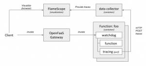
Functions in a Serverless environment (Tim Bray has a nice write-up of some of the key aspects of Serverless here. And let’s leave aside some side notes like this one.) like OpenFaaS or OpenWhisk are short lived things that really come and go. But wouldn’t it be useful to – regardless of this context – to be able to gain insight on how your functions perform? Hence being able to trace/profile the functions in an environment would be a nice to have add-on.
The following diagram shows a high-level overview of how this could look like.
 (Click to enlarge)
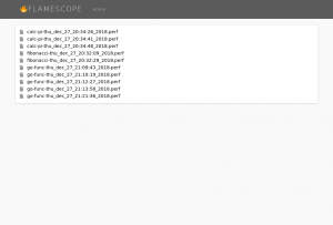
Once you have the tracing/profiling of your functions in place FlameScope is a handy tool to visualize them. Here you can see the list of trace for previously executed functions:
 (Click to enlarge)
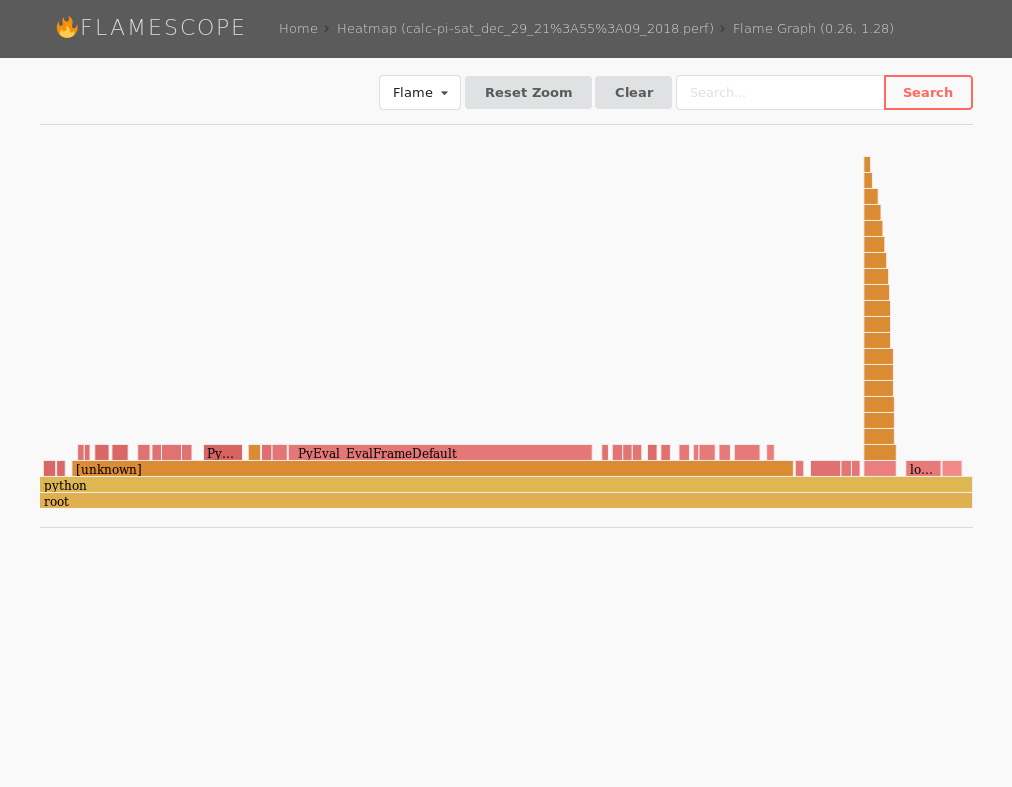
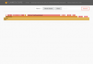
Drilling deeper into them you can see the actually FlameGraphs of each function – for example a function calculating pi.
 (Click to enlarge)
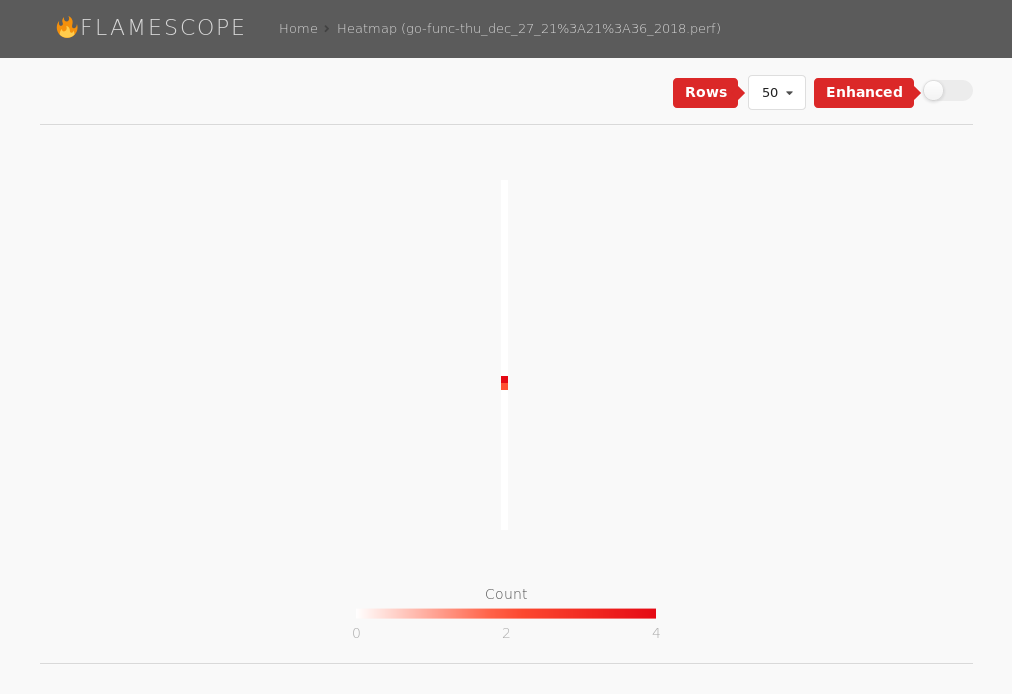
As some functions have a very short lifespan, you will also note – that by looking at the heatmaps – not a lot is going:
 (Click to enlarge)
I’m not necessarily claiming this is all very useful – especially since some functions are still very short lived, and their traces are not capturing a lot of information, therefore. However the general concept of all this sounds intriguing to me. Running your function on different platforms for example will results in difference in the FlameGraph. The function shown here will calculate Pi and perform some I/O operations for test purposes. The function’s FlameGraph from above looks a bit different when run on a different platform (Xeon vs i5):
 (Click to enlarge)
Multiple runs of the same function on the same platform will results in similar FlameGraphs.
The following sections describe how to enable such a scenario:
Step 1) enabling the environment
Frameworks such as OpenFaas or OpenWhisk will use docker [cold|warm|hot] containers to host the functions. So one of the initial steps it to enable tracing in those containers. By one some syscalls are blocked – for good reason – in docker [src]. Unless you want to go dig deep into OpenFaaS or OpenWhisk and change how they run containers, the easiest way forward it to enable e.g. the perf_event_open system call using seccomp security profiles system wide. To do so start dockerd with the following parameters:
$ sudo dockerd -H unix:///var/run/docker.sock --seccomp-profile /etc/docker/defaults.json
An example security profile can be found here. Just whitelist the right system calls that you will need and store the profile in /etc/docker/defaults.json. For this example we will user perf, hence we need to enable perf_event_open.
Note: another option (almost more elegant & more secure) would be to trace the functions not from within the container, but on the host system. perf does allow for limiting the cgroup and hence doing this (through the option –cgroup=docker/…) , but this would yet again require some more integration work with your framework. Also note that although perf does not add a lot of overhead for instrumentation, it also does not come “for free” either.
Step 2) plumbing
As we will trace the functions from within their containers, we need to get the data out of the containers. A simple python HTTP service that allows for POSTing traces to it, will also store the same into files in a directory. As this service can be run in a container itself, this directory can easily be mounted to the container. Now within each container we can simply post the data (in the file trace.perf) to the data collector:
$ curl -X POST http://172.17.0.1:9876/ -H 'X-name: go-func' --data-binary @trace.perf
Step 3) altering the templates
The easiest way to kick of the tracing command perf, whenever a function is executed is by altering the template of your framework. For OpenFaaS your can easily pull the templatest using:
$ faas-cli template pull
Once they have been pulled the easiest thing to do is to alter the Dockerfile to include a shell script which executes e.g. your perf commands:
#!/bin/sh

perf record -o perf.data -q -F 1004 -p $1 -a -g -- sleep 5
perf script -i perf.data --header > trace.perf
curl -X POST http://172.17.0.1:9876/ -H 'X-name: fibonacci' --data-binary @trace.perf
Note that in this example we use perf to instrument at a frequency of 1004 Hz – just offsetting it from 1000 Hz to make sure we capture everything. It might make sense to tweak the frequency according to your environment – 1000 Hz is already providing a lot of detail.
Also we need to alter the Dockerfiles to a) install the perf tool and b) ensure we can execute it with the user app:
...
RUN apk add curl sudo
RUN  apk add linux-tools --update-cache --repository http://dl-3.alpinelinux.org/alpine/edge/testing/ --allow-untrusted

# Add non root user
RUN addgroup -S app && adduser app -S -G app wheel
RUN adduser app wheel
RUN echo '%app ALL=(ALL) NOPASSWD:ALL' >> /etc/sudoers

WORKDIR /home/app/

# ensure we copy the trace file over as well.
COPY trace.sh           .
...
Also make sure that this shell script will get call whenever your function is triggered. For example in the python templates alter the index.py file, for e.g. golang edit the main.go file. Within those just execute the shell script above with the PID of the current process as the first argument
Step 4) visualize it
FlameGraphs are pretty handy, and a team @ Netflix (including Brendan Gregg) have been busy writing a handy tool to visualize the traces. FlameScope can easily be executed using a docker command:
$ docker run --rm -it -v /tmp/stacks:/stacks:ro -p 5000:5000 flamescope
Note: that I had to do some minor tweaks to get FlameScope to work. I had to update the Dockerfile to the python3 version of alpine, manually add libmagic (apk add libmagic), and don’t forget to configure FlameScope to pickup the profiles from /stacks in config.py.
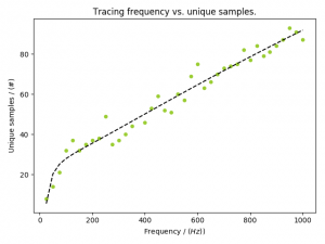
Update [2019/01/08] Originally I traced the functions with a frequency of 1004 Hz. This seems to be a bit high. As you can see in the following graph – and read this as a rule of thumb, not necessarily the ground truth – sampling at about 200 Hz will give you the necessary information:
 (Click to enlarge)
Categories: Personal • Tags: FaaS, Instrumentation, Orchestration, Serverless • Permalink for this article
April 15th, 2018 • Comments Off on Agent based bidding for merging graphs
There are multiple ways to merge two stitch two graphs together. Next to calculating all possible solutions or use evolutionarty algorithms bidding is a possible way.
The nodes in the container, just like in a Multi-Agent System [1], pursue a certain self-interest, as well as an interest to be able to stitch the request collectively. Using a english auction (This could be flipped to a dutch one as well) concept the nodes in the container bid on the node in the request, and hence eventually express a interest in for a stitch. By bidding credits the nodes in the container can hide their actually capabilities, capacities and just express as interest in the form of a value. The more intelligence is implemented in the node, the better it can calculate it’s bids.
The algorithm starts by traversing the container graph and each node calculates it’s bids. During traversal the current assignments and bids from other nodes are ‘gossiped’ along. The amount of credits bid, depends on if the node in the request graph matches the type requirement and how well the stitch fits. The nodes in the container need to base their bids on the bids of their surrounding environment (especially in cases in which the same, diff, share, nshare conditions are used). Hence they not only need to know about the current assignments, but also the neighbours bids.
For the simple lg and lt conditions, the larger the delta between what the node in the request graphs asks for (through the conditions) and what the node in the container offers, the higher the bid is. Whenever a current bid for a request node’s stitch to the container is higher than the current assignment, the same is updated. In the case of conditions that express that nodes in the request need to be stitched to the same or different container node, the credits are calculated based on the container node’s knowledge about other bids, and what is currently assigned. Should a pair of request node be stitched – with the diff conditions in place – the current container node will increase it’s bid by 50%, if one is already assigned somewhere else. Does the current container node know about a bid from another node, it will increase it’s bid by 25%.
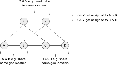
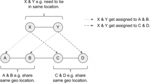
For example a container with nodes A, B, C, D needs to be stitched to a request of nodes X, Y. For X, Y there is a share filter defined – which either A & B, or C & D can fulfill. The following diagram shows this:
(Click to enlarge)
Let’s assume A bids 5 credits for X, and B bids 2 credits for Y, and C bids 4 credits for X and D bids 6 credits for Y. Hence the group C & D would be the better fit. When evaluating D, D needs to know X is currently assigned to A – but also needs to know the bid of C so is can increase it’s bid on Y. When C is revisited it can increase it’s bid given D has Y assigned. As soon as the nodes A & B are revisited they will eventually drop their bids, as they now know C & D can serve the request X, Y better. They hence sacrifice their bis for the needs of the greater good. So the fact sth is assigned to a neighbour matters more then the bid of the neighbour (increase by 50%) – but still, the knowledge of the neighbour’s bid is crucial (increase by 25%) – e.g. if bid from C would be 0, D should not bit for Y.
The ability to increase the bids by 25% or 50% is important to differentiate between the fact that sth is assigned somewhere else, or if the environment the node knows about includes a bid that can help it’s own bid.
Note this algorithm does not guarantee stability. Also for better results in specific use cases it is encourage to change how the credits are calculated. For example based on the utility of the container node. Especially for the share attribute condition there might be cases that the algorithm does not find the optimal solution, as the increasing percentages (50%, 25%) are not optimal. The time complexity depends on the number of nodes in the container graph, their structure and how often bids & assignment change. This is because currently the container graph is traversed synchronously. In future a async approach would be beneficial, which will also allow for parallel calculation of bids.
The bidding concept is implemented as part of the graph-stitcher tool.
Categories: Personal • Tags: Graph Stitching, Graphs, Python • Permalink for this article
November 18th, 2017 • Comments Off on Q-Learning in python
There is a nice tutorial that explains how Q-Learning works here. The following python code implements the basic principals of Q-Learning:
Let’s assume we have a state matrix defining how we can transition between states, and a goal state (5):
GOAL_STATE = 5
# rows are states, columns are actions
STATE_MATRIX = np.array([[np.nan, np.nan, np.nan, np.nan, 0., np.nan],
                         [np.nan, np.nan, np.nan, 0., np.nan, 100.],
                         [np.nan, np.nan, np.nan, 0., np.nan, np.nan],
                         [np.nan, 0., 0., np.nan, 0., np.nan],
                         [0., np.nan, np.nan, 0, np.nan, 100.],
                         [np.nan, 0., np.nan, np.nan, 0, 100.]])
Q_MATRIX = np.zeros(STATE_MATRIX.shape)
Visually this can be represented as follows:

(Click to enlarge)
For example if you are in state 0, we can go to state 4, define by the 0. . If we are in state 4, we can directly goto to state 5 define by the 100. . np.nan define impossible transitions. Finally we initialize an empty Q-Matrix.
Now the Q-Learning algorithm is simple. The comments in the following code segment will guide through the steps:
i = 0
while i < MAX_EPISODES:
    # pick a random state
    state = random.randint(0, 5)
    while state != goal_state:
        # find possible actions for this state.
        candidate_actions = _find_next(STATE_MATRIX[state])

        # randomly pick one action.
        action = random.choice(candidate_actions)

        # determine what the next states could be for this action...
        next_actions = _find_next(STATE_MATRIX[action])
        values = []
        for item in next_actions:
            values.append(Q_MATRIX[action][item])

        # add some exploration randomness...
        if random.random() < EPSILON:
            # so we do not always select the best...
            max_val = random.choice(values)
        else:
            max_val = max(values)

        # calc the Q value matrix...
        Q_MATRIX[state][action] = STATE_MATRIX[state][action] + \
                                  EPSILON * max_val

        # next step.
        state = action
    i += 1
We need one little helper routine for this – it will help in determine the next possible step I can do:
def _find_next(items):
    res = []
    i = 0
    for item in items:
        if item >= 0:
            res.append(i)
        i += 1
    return res
Finally we can output the results:
Q_MATRIX = Q_MATRIX / Q_MATRIX.max()

np.set_printoptions(formatter={'float': '{: 0.3f}'.format})
print Q_MATRIX
This will output the following Q-Matrix:
[[ 0.000  0.000  0.000  0.000  0.800  0.000]
 [ 0.000  0.000  0.000  0.168  0.000  1.000]
 [ 0.000  0.000  0.000  0.107  0.000  0.000]
 [ 0.000  0.800  0.134  0.000  0.134  0.000]
 [ 0.044  0.000  0.000  0.107  0.000  1.000]
 [ 0.000  0.000  0.000  0.000  0.000  0.000]]
This details for example the best path to get from e.g. state 2 to state 5 is: 2 -> 3 (0.107), 3 -> 1 (0.8), 1 -> 5 (1.0).
Categories: Personal • Tags: Machine Learning, Python • Permalink for this article
November 12th, 2017 • Comments Off on Controlling a Mesos Framework
Note: This is purely for fun, and only representing early results.
It is possible to combine more traditional scheduling and resource managers like OpenLava with DCOS like Mesos [1]. The basic implementation which glues OpenLava and Mesos together is very simple: as long as jobs are in the queue(s) of the HPC/HTC scheduler it will try to consume offers presented by Mesos to run these jobs on. There is a minor issue with that however: the framework is very greedy, and will consume a lot of offers from Mesos (So be aware to set quotas etc.).
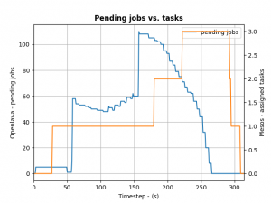
To control how many offers/tasks the Framework needs to dispatch the jobs in the queue of the HPC/HTC scheduler we can use a simple PID controller. By applying a bit of control we can tame the framework as the following the diagram shows:
(Click to enlarge)
We define the ratio between running and pending jobs as a possible target or the controller (Accounting for a division by zero). Given this, we can set the PID controller to try to keep the system at the ratio of e.g. 0.3 as a target (semi-randomly picked).
For example: if 10 jobs are running, while 100 are in the queue pending, the ratio will be 0.1 and we need to take more resource offers from Mesos. More offers, means more resources available for the jobs in the queues – so the number of running jobs will increase. Let’s assume a stable number of jobs in the queue, so e.g. the system will now be running 30 jobs and 100 jobs are in the queue. This represent the steady state and the system is happy. If the number of jobs in the queues decreases the system will need less resources to process them. For example 30 jobs are running, while 50 are pending gives us a ratio of 0.6. As this is a higher ratio than the specified target, the system will decrease the number of tasks needed from Mesos.
This approach is very agnostic to job execution times too. Long running jobs will lead to more jobs in the queue (as they are blocking resources) and hence decreasing the ratio, leading to the framework picking up more offers. Short running jobs will lead to the number of pending jobs decreasing faster and hence a higher ratio, which in turn will lead to the framework disregarding resources offered to it.
And all the magic is happening very few lines of code running in a thread:
def run(self):
    while not self.done:
        error = self.target - self.current  # target = 0.3, self.current == ratio from last step
        goal = self.pid_ctrl.step(error)  # call the PID controller
        self.current, pending = self.scheduler.get_current()  # get current ratio from the scheduler
        self.scheduler.goal = max(0, int(goal))  # set the new goal of # of needed tasks.
        time.sleep(1)
The PID controller itself is super basic:
class PIDController(object):
    """
    Simple PID controller.
    """

    def __init__(self, prop_gain, int_gain, dev_gain, delta_t=1):
        # P/I/D gains
        self.prop_gain = prop_gain
        self.int_gain = int_gain
        self.dev_gain = dev_gain

        self.delta_t = delta_t

        self.i = 0
        self.d = 0
        self.prev = 0

    def step(self, error):
        """
        Do some work & progress.
        """
        self.i += self.delta_t * error
        self.d = (error - self.prev) / self.delta_t
        self.prev = error

        tmp = \
            self.prop_gain * error + \
            self.int_gain * self.i + \
            self.dev_gain * self.d
        return tmp
I can recommend the following book on control theory btw: Feedback Control for Computer Systems.
Categories: Personal • Tags: Control Theory, LSF, Orchestration, Scheduling • Permalink for this article
Page 2 of 36«12345...102030...»Last »