April 15th, 2018 • Comments Off on Agent based bidding for merging graphs
There are multiple ways to merge two stitch two graphs together. Next to calculating all possible solutions or use evolutionarty algorithms bidding is a possible way.
The nodes in the container, just like in a Multi-Agent System [1], pursue a certain self-interest, as well as an interest to be able to stitch the request collectively. Using a english auction (This could be flipped to a dutch one as well) concept the nodes in the container bid on the node in the request, and hence eventually express a interest in for a stitch. By bidding credits the nodes in the container can hide their actually capabilities, capacities and just express as interest in the form of a value. The more intelligence is implemented in the node, the better it can calculate it’s bids.
The algorithm starts by traversing the container graph and each node calculates it’s bids. During traversal the current assignments and bids from other nodes are ‘gossiped’ along. The amount of credits bid, depends on if the node in the request graph matches the type requirement and how well the stitch fits. The nodes in the container need to base their bids on the bids of their surrounding environment (especially in cases in which the same, diff, share, nshare conditions are used). Hence they not only need to know about the current assignments, but also the neighbours bids.
For the simple lg and lt conditions, the larger the delta between what the node in the request graphs asks for (through the conditions) and what the node in the container offers, the higher the bid is. Whenever a current bid for a request node’s stitch to the container is higher than the current assignment, the same is updated. In the case of conditions that express that nodes in the request need to be stitched to the same or different container node, the credits are calculated based on the container node’s knowledge about other bids, and what is currently assigned. Should a pair of request node be stitched – with the diff conditions in place – the current container node will increase it’s bid by 50%, if one is already assigned somewhere else. Does the current container node know about a bid from another node, it will increase it’s bid by 25%.
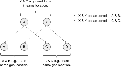
For example a container with nodes A, B, C, D needs to be stitched to a request of nodes X, Y. For X, Y there is a share filter defined – which either A & B, or C & D can fulfill. The following diagram shows this:
(Click to enlarge)
Let’s assume A bids 5 credits for X, and B bids 2 credits for Y, and C bids 4 credits for X and D bids 6 credits for Y. Hence the group C & D would be the better fit. When evaluating D, D needs to know X is currently assigned to A – but also needs to know the bid of C so is can increase it’s bid on Y. When C is revisited it can increase it’s bid given D has Y assigned. As soon as the nodes A & B are revisited they will eventually drop their bids, as they now know C & D can serve the request X, Y better. They hence sacrifice their bis for the needs of the greater good. So the fact sth is assigned to a neighbour matters more then the bid of the neighbour (increase by 50%) – but still, the knowledge of the neighbour’s bid is crucial (increase by 25%) – e.g. if bid from C would be 0, D should not bit for Y.
The ability to increase the bids by 25% or 50% is important to differentiate between the fact that sth is assigned somewhere else, or if the environment the node knows about includes a bid that can help it’s own bid.
Note this algorithm does not guarantee stability. Also for better results in specific use cases it is encourage to change how the credits are calculated. For example based on the utility of the container node. Especially for the share attribute condition there might be cases that the algorithm does not find the optimal solution, as the increasing percentages (50%, 25%) are not optimal. The time complexity depends on the number of nodes in the container graph, their structure and how often bids & assignment change. This is because currently the container graph is traversed synchronously. In future a async approach would be beneficial, which will also allow for parallel calculation of bids.
The bidding concept is implemented as part of the graph-stitcher tool.
Categories: Personal • Tags: Graph Stitching, Graphs, Python • Permalink for this article
November 18th, 2017 • Comments Off on Q-Learning in python
There is a nice tutorial that explains how Q-Learning works here. The following python code implements the basic principals of Q-Learning:
Let’s assume we have a state matrix defining how we can transition between states, and a goal state (5):
GOAL_STATE = 5
# rows are states, columns are actions
STATE_MATRIX = np.array([[np.nan, np.nan, np.nan, np.nan, 0., np.nan],
                         [np.nan, np.nan, np.nan, 0., np.nan, 100.],
                         [np.nan, np.nan, np.nan, 0., np.nan, np.nan],
                         [np.nan, 0., 0., np.nan, 0., np.nan],
                         [0., np.nan, np.nan, 0, np.nan, 100.],
                         [np.nan, 0., np.nan, np.nan, 0, 100.]])
Q_MATRIX = np.zeros(STATE_MATRIX.shape)
Visually this can be represented as follows:

(Click to enlarge)
For example if you are in state 0, we can go to state 4, define by the 0. . If we are in state 4, we can directly goto to state 5 define by the 100. . np.nan define impossible transitions. Finally we initialize an empty Q-Matrix.
Now the Q-Learning algorithm is simple. The comments in the following code segment will guide through the steps:
i = 0
while i < MAX_EPISODES:
    # pick a random state
    state = random.randint(0, 5)
    while state != goal_state:
        # find possible actions for this state.
        candidate_actions = _find_next(STATE_MATRIX[state])

        # randomly pick one action.
        action = random.choice(candidate_actions)

        # determine what the next states could be for this action...
        next_actions = _find_next(STATE_MATRIX[action])
        values = []
        for item in next_actions:
            values.append(Q_MATRIX[action][item])

        # add some exploration randomness...
        if random.random() < EPSILON:
            # so we do not always select the best...
            max_val = random.choice(values)
        else:
            max_val = max(values)

        # calc the Q value matrix...
        Q_MATRIX[state][action] = STATE_MATRIX[state][action] + \
                                  EPSILON * max_val

        # next step.
        state = action
    i += 1
We need one little helper routine for this – it will help in determine the next possible step I can do:
def _find_next(items):
    res = []
    i = 0
    for item in items:
        if item >= 0:
            res.append(i)
        i += 1
    return res
Finally we can output the results:
Q_MATRIX = Q_MATRIX / Q_MATRIX.max()

np.set_printoptions(formatter={'float': '{: 0.3f}'.format})
print Q_MATRIX
This will output the following Q-Matrix:
[[ 0.000  0.000  0.000  0.000  0.800  0.000]
 [ 0.000  0.000  0.000  0.168  0.000  1.000]
 [ 0.000  0.000  0.000  0.107  0.000  0.000]
 [ 0.000  0.800  0.134  0.000  0.134  0.000]
 [ 0.044  0.000  0.000  0.107  0.000  1.000]
 [ 0.000  0.000  0.000  0.000  0.000  0.000]]
This details for example the best path to get from e.g. state 2 to state 5 is: 2 -> 3 (0.107), 3 -> 1 (0.8), 1 -> 5 (1.0).
Categories: Personal • Tags: Machine Learning, Python • Permalink for this article
November 12th, 2017 • Comments Off on Controlling a Mesos Framework
Note: This is purely for fun, and only representing early results.
It is possible to combine more traditional scheduling and resource managers like OpenLava with DCOS like Mesos [1]. The basic implementation which glues OpenLava and Mesos together is very simple: as long as jobs are in the queue(s) of the HPC/HTC scheduler it will try to consume offers presented by Mesos to run these jobs on. There is a minor issue with that however: the framework is very greedy, and will consume a lot of offers from Mesos (So be aware to set quotas etc.).
To control how many offers/tasks the Framework needs to dispatch the jobs in the queue of the HPC/HTC scheduler we can use a simple PID controller. By applying a bit of control we can tame the framework as the following the diagram shows:
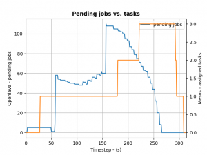
(Click to enlarge)
We define the ratio between running and pending jobs as a possible target or the controller (Accounting for a division by zero). Given this, we can set the PID controller to try to keep the system at the ratio of e.g. 0.3 as a target (semi-randomly picked).
For example: if 10 jobs are running, while 100 are in the queue pending, the ratio will be 0.1 and we need to take more resource offers from Mesos. More offers, means more resources available for the jobs in the queues – so the number of running jobs will increase. Let’s assume a stable number of jobs in the queue, so e.g. the system will now be running 30 jobs and 100 jobs are in the queue. This represent the steady state and the system is happy. If the number of jobs in the queues decreases the system will need less resources to process them. For example 30 jobs are running, while 50 are pending gives us a ratio of 0.6. As this is a higher ratio than the specified target, the system will decrease the number of tasks needed from Mesos.
This approach is very agnostic to job execution times too. Long running jobs will lead to more jobs in the queue (as they are blocking resources) and hence decreasing the ratio, leading to the framework picking up more offers. Short running jobs will lead to the number of pending jobs decreasing faster and hence a higher ratio, which in turn will lead to the framework disregarding resources offered to it.
And all the magic is happening very few lines of code running in a thread:
def run(self):
    while not self.done:
        error = self.target - self.current  # target = 0.3, self.current == ratio from last step
        goal = self.pid_ctrl.step(error)  # call the PID controller
        self.current, pending = self.scheduler.get_current()  # get current ratio from the scheduler
        self.scheduler.goal = max(0, int(goal))  # set the new goal of # of needed tasks.
        time.sleep(1)
The PID controller itself is super basic:
class PIDController(object):
    """
    Simple PID controller.
    """

    def __init__(self, prop_gain, int_gain, dev_gain, delta_t=1):
        # P/I/D gains
        self.prop_gain = prop_gain
        self.int_gain = int_gain
        self.dev_gain = dev_gain

        self.delta_t = delta_t

        self.i = 0
        self.d = 0
        self.prev = 0

    def step(self, error):
        """
        Do some work & progress.
        """
        self.i += self.delta_t * error
        self.d = (error - self.prev) / self.delta_t
        self.prev = error

        tmp = \
            self.prop_gain * error + \
            self.int_gain * self.i + \
            self.dev_gain * self.d
        return tmp
I can recommend the following book on control theory btw: Feedback Control for Computer Systems.
Categories: Personal • Tags: Control Theory, LSF, Orchestration, Scheduling • Permalink for this article
April 17th, 2017 • Comments Off on Distributed systems: which cluster do I obey?
The topic of cluster formation in itself is not new. There are plenty of methods around to form cluster on the fly [1]. They mostly follow methods which make use of gossip protocols. Implementation can wildly be found, even in products like Akka.
Once a cluster is formed the question becomes wehter control (see this post for some background) is centralized or decentralized. Or something in between with a (hierarchical) set of leaders managing – in a distributed fashion – a cluster of entities that are actuating. Both, centralized and decentralized approaches, have their advantages and disadvantages. Centralized approaches are sometimes more efficient as they might have more knowledge to base their decisions upon. Note that even in centralized management approaches a gossip protocols might be in use. There are also plenty of algorithms around to support consensus and leader election [2], [3].
Especially in Fog and Fdge computing use cases, entities which move (e.g. a car, plane, flying/sailing drone) have to decide to which cluster they want to belong and obey the actions initiated by those. Graph representations are great for this – and yet again because of a rich set of algorithms in the graph theory space, the solution might be quite simple to implement. Note that in Fog/Edge use cases there most likely will always be very (geographic) static entities like Cloudlets in the mix – which could be elected as leaders.
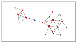
For example, the following diagram shows two clusters: The red nodes’ size indicates who is the current leader. The blue dot – marks an entity that is connected to both clusters. The width of the edge connecting it to the cluster indicates to which cluster it ‘belongs’ (aka it’s affinity).
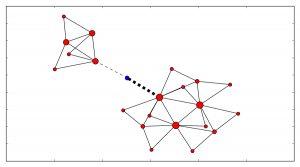
(Click to enlarge)
Now as the blue entity moves (geographically) the connections/edges to the clusters change. Now based on algorithms like this, the entity can make a decision to hand-off control to another cluster and obey the directions given from it.
(Click to enlarge)
Categories: Personal • Tags: Distributed Systems, Graphs • Permalink for this article
January 7th, 2017 • Comments Off on Example 2: Intelligent Orchestration & Scheduling with OpenLava
This is the second post in a series (the first post can be found here) about how to insert smarts into a resource manager. So let’s look how a job scheduler or distributed resource management system (DRMS) — in a HPC use case — with OpenLava can be used. For the rationale behind all this check the background section of the last post.
The basic principle about this particular example is simple: each host in a cluster will report a “rank”; the rank will be used to make a decision on where to place a job. The rank could be defined as: a rank is high when the sub-systems of the hosts are heavily used; and the rank is low when none or some sub-system are utilized. How the individual sub-systems usage influences the rank value, is something that can be machine learned.
Let’s assume the OpenLava managed cluster is up and running and a couple of hosts are available. The concept of elims can be used to get the job done. The first step is, to teach the system what the rank is. This is done in the lsf.shared configuration file. The rank is defined to be a numeric value which will be updated every 10 seconds (while not increasing):
Begin Resource
RESOURCENAME  TYPE    INTERVAL INCREASING  DESCRIPTION
   ...
   rank       Numeric 10       N           (A rank for this host.)
End Resource
Next OpenLava needs to know for which hosts this rank should be determined. This is done through a concept of ‘resource mapping’ in the lsf.cluster.* configuration file. For now the rank should be used for all hosts by default:
Begin ResourceMap
RESOURCENAME LOCATION
rank ([default])
End ResourceMap
Next an external load information manager (LIM) script which will report the rank to OpenLava needs to be written. OpenLava expects that the script writes to stdout with the following format: <number of resources to report on> <first resource name> <first resource value> <second resource name> <second resource value> … . So in this case it should spit out ‘1 rank 42.0‘ every 10 seconds. The following python script will do just this – place this script in the file elim in $LSF_SERVERDIR:
#!/usr/bin/python2.7 -u

import time

INTERVAL = 10


def _calc_rank():
    # TODO calc value here...
    return {'rank': value}

while True:
    RES = _calc_rank()
    TMP = [k + ' ' + str(v) for k, v in RES.items()]
    print(\"%s %s\" % (len(RES), ' '.join(TMP)))
    time.sleep(INTERVAL)
Now a special job queue in the lsb.queues configuration file can be used which makes use of the rank. See the RES_REQ parameter in which it is defined that the candidate hosts for a job request are ordered by the rank:
Begin Queue
QUEUE_NAME = special
DESCRIPTION = Special queue using the rank coming from the elim.
RES_REQ = order[rank]
End Queue
Submitting a job to this queue is as easy as: bsub -q special sleep 1000. Or the rank can be passed along as a resource requirements on job submission (for any other queue): bsub -R “order[-rank]” -q special sleep 1000. By adding the ‘-‘ it is said that the submitter request the candidate hosts to be sorted for hosts with a high rank first.
Let’s assume a couple of hosts are up & running and they have different ranks (see the last column):
openlava@242e2f1f935a:/tmp$ lsload -l
HOST_NAME               status  r15s   r1m  r15m   ut    pg    io  ls    it   tmp   swp   mem   rank
45cf955541cf                ok   0.2   0.2   0.3   2%   0.0     0   0 2e+08  159G   16G   11G    9.0
b7245f8e6d0d                ok   0.2   0.2   0.3   2%   0.0     0   0 2e+08  159G   16G   11G    8.0
242e2f1f935a                ok   0.2   0.2   0.3   3%   0.0     0   0 2e+08  159G   16G   11G   98.0
When checking the earlier submitted job, the execution host (EXEC_HOST) is indeed the hosts with the lowest rank as expected:
openlava@242e2f1f935a:/tmp$ bjobs
JOBID   USER    STAT  QUEUE      FROM_HOST   EXEC_HOST   JOB_NAME   SUBMIT_TIME
101     openlav RUN   special    242e2f1f935 b7245f8e6d0 sleep 1000 Jan  7 10:06
The rank can also be seen in web interface like the one available for the OpenLava Mesos framework. What was described in this post is obviously just an example – other methods to integrate your smarts into the OpenLava resource manager can be realized as well.
Categories: Personal • Tags: LSF, Orchestration, Scheduling, SDI • Permalink for this article
Page 3 of 24«12345...1020...»Last »